10/16/2026 – Climate- Science.press

Deep Magma’s Hidden Oxygen Cache May Have Helped Turn Earth Blue

A new study shows that silicate magma (molten rock) in Earth’s deep interior can store substantial “excess oxygen” beyond conventional chemical (stoichiometric) limits, acting like a volatile that is released upon ascent and potentially helping oxidize the shallow Earth and atmosphere.

It proposes a previously unrecognized geological mechanism that could have helped oxygenate Earth’s atmosphere, linking deep- mantle melting events to surface oxidation, especially around the time of the Great Oxidation Event.

A vivid digital illustration of a volcanic eruption, showcasing lava bubbling up through a cracked surface, with jets of blue water and steam rising from the fiery core against a dramatic sky. — AI generated by Grok

The research, published in National Science Review (DOI: 10.1093/nsr/nwag539) and announced by Science China Press (via EurekAlert, 15 October 2026), was led by Dr. Yanhao Lin and Dr. Ho-kwang Mao (Center for High Pressure Science and Technology Advanced Research / HPSTAR), with collaborators including Prof. Haiyang Niu (Northwestern Polytechnical University) and Prof. Wim van Westrenen (Vrije Universiteit Amsterdam).

Key findings

Traditionally, oxygen in magma was assumed to be fixed solely by the amounts and valence states of cations (Si, Mg, Fe, etc.). Unlike H₂O or CO₂, it was not treated as an independent volatile.
High -pressure and high- temperature experiments melted synthetic mid- ocean ridge basalt at 1 atm to 7 GPa (depths of hundreds of km) and 1200- 1800 °C, using an oxygen source (PtO₂). After quenching to glass, researchers measured major elements, H₂O, and CO₂, then calculated residual “excess oxygen” after accounting for stoichiometric needs and oxygen bound in water and CO₂.
Excess oxygen was near zero at 1 atm but rose to >5 wt% at 7 GPa. Controls without PtO₂ showed only 0.2- 0.5 wt%. Raman spectroscopy indicated the excess is incorporated into the melt and glass structure (not free O₂ bubbles). Measured amounts are likely lower limits due to possible loss during quenching.⁠
Molecular dynamics simulations (using deep neural network potentials with ab initio accuracy) on a simplified Mg- Si- O system reproduced the pressure- dependent uptake. As oxygen content rises, oxygen charges become more variable and some peroxide- like O–O bonds form, allowing storage beyond traditional limits. Capacity increases with pressure in a manner analogous to H₂O and CO₂ solubility.

Implications for Earth’s atmosphere

Magma generated in oxidized deep- mantle regions could carry excess oxygen. As it rises and pressure drops, solubility decreases and O₂ is released, potentially oxidizing the shallow mantle, crust, and atmosphere. This offers a direct physical link between deep melting and surface oxidation.⁠

The timing aligns with major atmospheric oxygen rises ~2.5- 2.0 billion years ago (Great Oxidation Event and aftermath), which overlapped with some of Earth’s largest large igneous provinces (LIPs) from deep-sourced magmatism. A rough estimate indicates that release of only ~0.27 wt% excess oxygen from magma erupted in that period could account for all the oxygen in today’s atmosphere.⁠

The work reframes magma as an active, pressure- sensitive reservoir in planetary oxygen cycles. It has implications for magma- ocean evolution, volatile degassing, atmospheric evolution on Earth, and long- term habitability of other terrestrial planets.⁠

This is a recent experimental and computational result proposing a previously unrecognized mechanism; it complements (rather than replaces) other processes involved in Earth’s oxygenation history, such as biological photosynthesis, changes in volcanic gas composition, and subduction- related recycling.

Diagram illustrating the Earth's interior layers, including the oxygenated mantle, ultra-low velocity zones (ULVZ), and the iron core, with arrows indicating convection and heat flow. — Schematic cross- section of Earth’s mantle. Magma formed in a deep, oxygen- rich region of the mantle carries excess oxygen upward. As the magma rises and pressure drops, excess oxygen is released (blue dots), which could oxidize the shallow mantle, the crust and the atmosphere. LIP: large igneous province; ULVZ: ultra- low velocity zone. Credit: Science China Press

Core idea

Silicate magma deep in the Earth can dissolve substantial “excess” (non- stoichiometric) oxygen as a pressure- dependent volatile, near zero at surface pressure but rising to more than ~5 wt% at pressures above ~5 GPa (hundreds of kilometers depth).

When this oxygen- rich magma rises and pressure drops, the excess oxygen is released as O₂. This provides a direct pathway for transporting oxidizing power from the deep interior to the shallow mantle, crust, and atmosphere.

Relevance to Earth’s history

Timing with atmospheric oxygen rise: Major increases in atmospheric oxygen roughly 2.5- 2.0 billion years ago (the Great Oxidation Event and its aftermath) overlap with the emplacement of some of Earth’s largest large igneous provinces (LIPs)—massive volcanic outpourings fed by deep mantle plumes. The new mechanism offers a physical link between these deep magmatic events and surface oxidation.⁠
Scale of the effect: A rough estimate in the study indicates that if magma erupted during that period released just ~0.27 wt% excess oxygen, the total amount liberated could equal all the oxygen present in today’s atmosphere. Experimental storage capacities at high pressure are an order of magnitude higher, so even partial degassing could have been geologically significant.⁠
Broader oxygen cycle: Magma is reframed as an active, dynamic reservoir in planetary oxygen cycles rather than a passive carrier of fixed chemistry. This complements (does not replace) other well-known factors in Earth’s oxygenation history, such as:
- Biological oxygen production by cyanobacteria (photosynthesis).
- Changes in the redox state of volcanic gases.
- Burial of organic carbon.
- Subduction and recycling of oxidized surface materials.
- Earlier processes such as iron disproportionation in magma oceans that oxidized the mantle after core formation.

Additional historical and planetary implications

It supplies a new way to evaluate early Earth magma- ocean evolution and volatile degassing.
The same physics could apply to other rocky planets, affecting whether they develop or retain oxygen- rich atmospheres and long- term habitability.
It highlights how deep interior processes can influence surface conditions over billions of years, reinforcing the interconnected nature of Earth’s interior- surface- atmosphere system.

In short, the finding does not overturn the biological or surface- driven explanations for the rise of oxygen, but it adds a plausible deep- Earth contribution that helps explain the coincidence of major atmospheric oxygen increases with large-scale mantle melting events in the Paleoproterozoic. It is a recent experimental and computational result (published 2026 in National Science Review), so further work will test how quantitatively important this process was relative to other mechanisms.

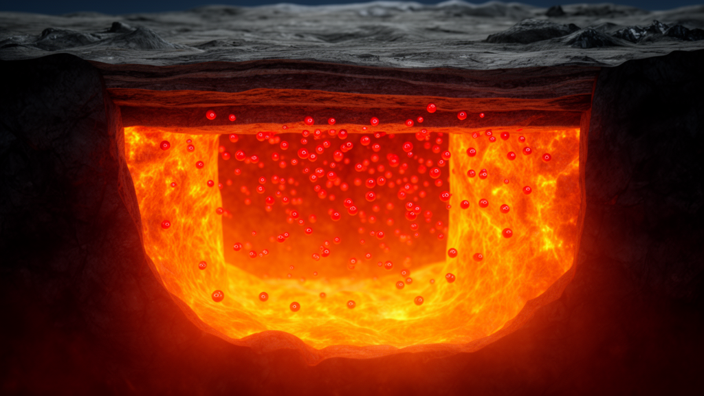
A cross-section view of the Earth's interior showing a magma chamber filled with glowing molten lava and gas bubbles. — https://scienmag.com/wp-content/uploads/2026/10/stackrss-featured-15740.png

Magma as a carrier of non- stoichiometric oxygen linking Earth’s interior and atmosphere

This is the full open- access research article corresponding to the news story discussed earlier.

Abstract (key points)

Magma generation and transport govern planetary evolution. Although oxygen is the most abundant anion in Earth’s silicate interior, its role in magma has conventionally been ignored, with oxygen contents assumed to be fixed solely by cation stoichiometry.

High- pressure and high- temperature experiments combined with molecular dynamics simulations demonstrate that silicate magma can incorporate substantially more oxygen than traditional valence- state constraints allow. This “excess oxygen” behaves as a previously unrecognized volatile component: its concentration rises from near zero at 1 atm to > ∼5 wt% above 5 GPa, more than five times the maximum oxygen increase possible in Earth’s solid mantle via iron redox changes.

As oxygen- rich magmas ascend and decompress, their capacity to hold excess oxygen decreases, driving release of O₂. This provides a direct mechanism potentially linking mantle melting to oxidation of Earth’s shallow interior and atmosphere and identifies magma as a dynamic reservoir in planetary oxygen cycles.

Context from the study and press coverage

Experiments used synthetic mid- ocean ridge basalt melted at 1 atm, 7 GPa and 1200- 1800 °C (with PtO₂ as an oxygen source). Excess oxygen was quantified in quenched glasses after accounting for stoichiometric requirements plus H₂O and CO₂. Values exceed 5 wt% at the highest pressures; controls without the oxygen source showed only 0.2- 0.5 wt%. Raman data indicate structural incorporation rather than free O₂ bubbles.
Simulations (deep neural-network potentials) on a simplified Mg- Si- O system reproduce the pressure- dependent uptake and show broader oxygen charge distributions plus some peroxide- like O–O bonds.
Implications include a possible contribution to atmospheric oxygenation ~2.5–2.0 billion years ago (Great Oxidation Event period), overlapping with major large igneous provinces. Rough estimates suggest release of only ~0.27 wt% excess oxygen from relevant magmas could supply the amount of O₂ in the modern atmosphere.
Broader relevance: magma- ocean evolution, volatile degassing, and habitability of terrestrial planets.

The article is short (9 pages). The publisher page (academic.oup.com) and institutional repositories (e.g., Vrije Universiteit Amsterdam) host it under the open- access license.

Journal: National Science Review, Volume 13, Issue 18, Article nwag539

DOI: 10.1093/nsr/nwag539

License: Creative Commons Attribution 4.0 (open access)

Provided: Science China Press

Authors: Yongjiang Xu,

Arctic Winter Ice Set to Vanish Faster Than Thought, Ancient Algae Reveal

Future Arctic winter sea ice is projected to shrink by roughly 1 million km² more than earlier estimates suggested. This comes from a recent study (reported in Nature Geoscience) that used mid- Holocene paleoclimate data (~6,000 years ago) to better constrain and weight climate models.

Greater winter ice loss could amplify mid- latitude impacts already linked to reduced winter SIE, including colder and wetter winters in parts of Eurasia and North America, altered storm tracks, and extreme precipitation.

Scenic view of Arctic ice floes at sunset, depicting melting ice in a vast ocean landscape, with the text overlay: 'Arctic Winter Ice Set to Vanish Faster Than Thought, Ancient Algae Reveal.' — AI generated by Grok

Future Arctic winter sea ice is projected to shrink by roughly 1 million km² more than earlier estimates suggested. This comes from a recent study (reported in Nature Geoscience) that used mid- Holocene paleoclimate data (~6,000 years ago) to better constrain and weight climate models.

Researchers from the University of Cambridge and Mexico’s Centro de Investigación en Matemáticas compiled the largest database yet of a key biomarker produced by sea- ice algae, extracted from ocean sediment cores.

During the mid- Holocene, orbital changes caused warmer Arctic conditions and reduced sea ice, providing an independent “out- of- sample” test of how models handle warmer climates comparable to projected future greenhouse- gas forcing.

Models generally over- predicted the amount of winter sea ice that should have existed under those past conditions. By weighting the models according to how well they matched the paleodata (and historical observations), the positive bias was largely eliminated. This also narrowed projection uncertainty by as much as 85%.⁠

When the same weights were applied to future scenarios (SSP1/SSP2/SSP5), the multi- model mean winter sea- ice extent for 2090- 2099 came out consistently lower, by about 4- 6%, than the unweighted average. The extra loss is concentrated in regions such as the Barents, Greenland, and Labrador Seas, with possible ice- edge shifts of several degrees of latitude.

Why it matters

Winter ice sets the stage for the rest of the seasonal cycle; underestimating its retreat also understates effects on ocean circulation, regional weather, and the timing of summer melt.
The revised projections hint at larger knock- on impacts, including potentially more snowfall over southeast Greenland and more rainfall in the Mediterranean, with implications for ice- sheet stability and flood risk in southern Europe.
Winter conditions in the UK and across Europe could therefore be affected more than previously expected.⁠

In short, paleoclimate evidence from a naturally warmer Arctic indicates that standard climate models have been too conservative about future winter sea- ice loss. The study emphasizes that past warm periods can provide stronger constraints on model reliability than the relatively short instrumental record alone.

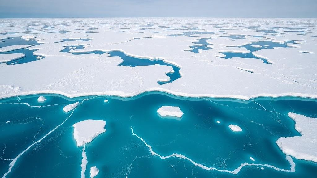
Aerial view of ice-covered ocean with patches of turquoise water and floating icebergs. — https://scienmag.com/wp-content/uploads/2026/10/stackrss-featured-16282.png

Palaeoclimate constraints narrow uncertainty in future Arctic winter sea ice projections

This is the peer- reviewed scientific paper underlying the recent news reports about greater- than- expected future Arctic winter sea- ice loss.

Key findings

Climate models show their largest biases and uncertainties for Arctic sea ice in winter (especially March), when ice cover strongly influences air- sea heat exchange, ocean mixing, and atmospheric circulation.

The authors address this by compiling the largest Arctic-wide database of mid- Holocene (MH; 5- 7 thousand years ago) sea- ice biomarkers (46 ln(PIP₂₅) observations based on the IP₂₅ biomarker and associated phytoplankton sterols from sediment cores spanning ~54- 83° N).

They use a Bayesian proxy system model (BaySIC) to translate model- simulated sea- ice concentrations into the same proxy units, accounting for non- stationary proxy seasonality (tied to local ice-breakup timing rather than fixed calendar months). A Bayesian weighting scheme then adjusts the contribution of each of 27 PMIP3/PMIP4 and CMIP models based on how well they match the MH proxies (and, in a joint analysis, historical observations). The scheme also accounts for model interdependence.

The weighted multi- model mean (WMMM) eliminates the positive winter sea- ice extent (SIE) bias and reduces uncertainty by ~85% (≈6.3 million km²), bringing it down to the level of interannual variability.
Applying the same weights to future projections (SSP1/SSP2/SSP5, corresponding to RCP2.6/4.5/8.5) yields winter SIE that is consistently ~4- 6% lower than the unweighted multi- model mean for 2090- 2099, nearly 1 million km² lower across scenarios.
Spatially, the weighted projections show higher probabilities of ice loss (and northward ice- edge shifts of up to 5.5° latitude) in the Barents, Greenland, and Labrador Seas.

Implications

The revised projections suggest late- winter and early- spring snowfall over southeastern Greenland may be underestimated by >30%, and Mediterranean winter, spring precipitation could be roughly twice as high as previously projected under high- emissions scenarios, with consequences for Greenland Ice Sheet mass balance and flood risk.

The mid- Holocene provides a particularly useful out- of- sample test because orbital changes produced Arctic radiative forcing comparable in magnitude (though different in seasonality and mechanism) to anticipated future greenhouse -gas forcing. Models that perform well under those past warm conditions are expected to be more reliable for future projections.

In short, quantitative palaeoclimate constraints from a warmer Arctic indicate that standard multi- model estimates have been too conservative about the magnitude of future winter sea-ice retreat and its cascading effects.

Journal: Nature Geoscience

DOI: 10.1038/s41561-026-02123-w

Published: 16 October 2026

Provided: University of Cambridge

Authors: C. Y. Fu,
M. B. Osman &
M. A. Aquino-López

Abstract

Arctic sea ice decline has been observed across all seasons and is projected to continue in the future. Relative to historical observations, climate models show their largest biases and uncertainties during winter, when ice cover strongly regulates air–sea heat exchange, ocean mixing and atmospheric circulation. Palaeoclimate records offer opportunities to evaluate model performance beyond the historical period, but applications have remained largely qualitative. Here we compile an Arctic-wide database of mid-Holocene (5–7 thousand years ago) biomarkers to assess sea ice simulations of this past warm period. Using a recently developed proxy system model, we present a Bayesian palaeoclimate model weighting scheme that refines the multi-model mean winter sea ice extent through fully quantitative proxy-model comparisons, accounting for model interdependence and non-stationary proxy seasonality. We demonstrate that, by adjusting the contribution of each model to the ensemble mean based on proxy evidence, model weights can eliminate biases and reduce uncertainties by 85%, to the level of interannual variability. Weighted projections using the same climate models indicate that future winter sea ice extent may be nearly 1 million km² lower than prior estimates across forthcoming decades and possible emissions scenarios, with broad implications for Arctic ecosystems, mid-latitude weather, and cryosphere stability.

Wrong Media, Climate Central’s Claim of ‘Supercharged’ Hurricane Isaias Is False

On October 9th, as Hurricane Isaias closed in on the coast, Climate Central put out a rapid attribution analysis saying human-caused warming had heated the water under the storm and added about 7 mph to its winds.

Climate Central’s claim was carried by WSMV-TV and many other media outlets.

That same day, a reader asked Chris Martz about a claim attributed to Al Roker, that Isaias was fueled by a Gulf running 5 to 6 degrees above normal. Climate Realism was unable to find the claim online. It probably occurred during a TV segment.

The story you just read is true. Only the name of the Gulf has been changed.

Infographic debunking Climate Central's claim that Hurricane Isaias was 'Supercharged', highlighting that it was a Category 1 hurricane with no unusual intensification. — AI generated by Meta

From ClimateRealism

By Anthony Watts

Screenshot of an article discussing how climate change is affecting hurricane activity, featuring the text 'BOGUS' overlaid on the image.

EDITORS NOTE:

Climate Central’s claim was carried by WSMV-TV and many other media outlets.

Chris, a friend of Climate Realism, answered with data. His post follows, with a few notes added by Charles Rotter from WUWT. Chris Martz says:

Al Roker is not an actual meteorologist.

But I am.

You ask a really good question. And while Roker has opinions, I have data.

Yes, it is true that tropical cyclones (TCs) operate as thermodynamic heat engines sustained by ocean-to-atmosphere enthalpy fluxes, including sensible and latent heat transfer, with latent heat released during condensation, which maintain the deep convection. The higher the sea surface temperatures (SSTs) are, the higher the likelihood for TC intensification.

However, SST anomalies represent departures from climatological averages rather than absolute SSTs. That means below-average SSTs can still support an intense hurricane. In fact, the Gulf of Mexico (or Gulf of America; call it whatever you want) is warm enough during late August, September, and early October every year to support a hurricane of category four or five strength. That has always been the case and it always will be.

Al Roker is not an actual meteorologist.

But I am.

You ask a really good question. And while Roker has opinions, I have data.

Yes, it is true that tropical cyclones (TCs) operate as thermodynamic heat engines sustained by ocean-to-atmosphere enthalpy fluxes, including… https://t.co/oOBj677H0U pic.twitter.com/vBZ3WW5iK5
— Chris Martz (@ChrisMartzWX) October 10, 2026

That’s the whole argument in one paragraph. An anomaly is a departure from average. It isn’t the temperature, and the Gulf in September is never short of fuel.

I hypothesized that Gulf SSTAs don’t really affect TC strength as commonly claimed because of this fact. So, I decided to investigate this question to provide a numerical answer. All science is numbers.

For this analysis, I decided to use the NOAA National Hurricane Center’s (NHC) HURDAT2 database, which contains historical TC tracks (coordinates), maximum sustained wind speeds (Vmax), and pressures, which contains data spanning 1851 to 2025. I then employed the Extended Reconstructed Sea Surface Temperature (ERSSTv5) dataset from NOAA, which contains monthly SST estimates on a 2° × 2° grid since January 1854. So, my analysis must be restricted from 1854 to 2025.

I identified 269 TCs that attained hurricane strength (≥64 kt / ≥74 mph) within the Gulf during the study period. Of this subset, 70 originated within the Gulf itself, while the remaining 199 developed elsewhere, primarily in the Atlantic or the Caribbean Sea, before entering the Gulf. For each hurricane, I determined its highest Vmax while inside the Gulf specifically. I then compared that intensity against the mean SSTA (calculated by evaluating SST departures from the 1991–2020 baseline) sampled along its Gulf track, using the monthly ERSSTv5 data.

Monthly SST data is not perfect, but it provides us a fairly good estimate because water has a high heat capacity, meaning it takes a lot of energy gain in order to warm a body of water and a lot of energy loss to cool it. In layman terms, SSTs are usually rather slow to change from week-to-week.

Al Roker is not an actual meteorologist.

But I am.

You ask a really good question. And while Roker has opinions, I have data.

Yes, it is true that tropical cyclones (TCs) operate as thermodynamic heat engines sustained by ocean-to-atmosphere enthalpy fluxes, including… https://t.co/oOBj677H0U pic.twitter.com/vBZ3WW5iK5
— Chris Martz (@ChrisMartzWX) October 10, 2026

Both datasets are NOAA’s and both are public. Available to everyone.

The results show essentially no linear relationship between Gulf SST anomalies and the maximum sustained wind speeds attained by hurricanes within the basin.

Across all 269 Gulf hurricanes, the Pearson correlation coefficient was just r = +0.036, which indicates an extremely weak positive correlation. The coefficient of determination (R²) was 0.001, meaning that variations in SST anomalies explained approximately 0.1% of the observed variation in peak hurricane intensity under a simple linear regression model. The Spearman rank correlation coefficient was similarly negligible at ρ = +0.012. Furthermore, the Pearson correlation yielded a p-value of 0.555, well above the conventional statistical significance threshold of 0.05.

Therefore, the observed relationship is not statistically significant.

Al Roker is not an actual meteorologist.

But I am.

You ask a really good question. And while Roker has opinions, I have data.

Yes, it is true that tropical cyclones (TCs) operate as thermodynamic heat engines sustained by ocean-to-atmosphere enthalpy fluxes, including… https://t.co/oOBj677H0U pic.twitter.com/vBZ3WW5iK5
— Chris Martz (@ChrisMartzWX) October 10, 2026

An R² of 0.001. Departures from normal account for about a tenth of one percent of how strong Gulf hurricanes get.

The scatterplot below illustrates this quite clearly. Hurricanes attaining relatively modest maximum intensities of 65–85 kt occurred across a broad range of SSTAs, as did much stronger hurricanes exceeding 100–120 kt. Some of the most intense hurricanes in the dataset occurred during periods when SSTs along their Gulf tracks were below the 1991–2020 average. Conversely, some hurricanes traversing anomalously warm waters never intensified beyond minimal hurricane strength.

In layman terms? An anomalously warm Gulf has no meaningful correlation to Gulf hurricane intensity.

Al Roker is not an actual meteorologist.

But I am.

You ask a really good question. And while Roker has opinions, I have data.

Yes, it is true that tropical cyclones (TCs) operate as thermodynamic heat engines sustained by ocean-to-atmosphere enthalpy fluxes, including… https://t.co/oOBj677H0U pic.twitter.com/vBZ3WW5iK5
— Chris Martz (@ChrisMartzWX) October 10, 2026

Scatter plot showing the relationship between sea surface temperature anomaly and the highest sustained wind speed of Gulf of Mexico hurricanes from 1854 to 2025. The plot includes points for Gulf-origin and outside-origin storms, with a linear best fit line indicated. — https://x.com/ChrisMartzWX/status/2108781894368137294?s=20

The story you just read is true. Only the name of the Gulf has been changed.

Global Survey of 15,000 Ice Cliffs Challenges Theory of Accelerated Sea-Level Rise

A new study led by Woods Hole Oceanographic Institution (WHOI), published in Science on or around October 15, 2026, provides the most comprehensive observational analysis of ice cliffs at the margins of Earth’s ice sheets (primarily Antarctica and Greenland).

Marine ice- cliff instability (MICI) is a hypothesized process in which tall, near- vertical ice cliffs at the edges of marine- terminating glaciers or ice sheets become structurally unstable and collapse under their own weight, potentially triggering rapid, self- sustaining retreat of the ice sheet.

A serene landscape featuring towering ice cliffs beside a tranquil sea, under the glow of the aurora borealis, with a headline overlay regarding a global survey of ice cliffs and sea-level rise. — AI generated by Grok

A new study led by Woods Hole Oceanographic Institution (WHOI), published in Science on or around October 15, 2026, provides the most comprehensive observational analysis of ice cliffs at the margins of Earth’s ice sheets (primarily Antarctica and Greenland).

Researchers, including lead author Caroline Needell (MIT- WHOI Joint Program doctoral student), Catherine Walker (WHOI), and Jeremy Bassis (University of Michigan), analyzed 15,330 individual satellite observations (mainly from NASA’s ICESat- 2 laser altimetry, plus some earlier airborne data).

These measured cliff heights, ice thickness, water depth, crevassing, calving rates, and how fronts evolved over time (often in ~3- month intervals over multi- year periods).

Marine Ice- Cliff Instability (MICI)

MICI is a long- debated theory proposing that ice cliffs taller than roughly 100 m above the waterline can become structurally unstable under their own weight. Collapse would expose even taller inland ice, potentially trigger rapid, self- sustaining retreat and substantially accelerate sea- level rise contributions from ice sheets. It has featured in some of the highest sea- level projections but has never been directly observed in a runaway form, leading to debate over its inclusion in models.

Key Findings

Tall ice cliffs (>~90- 100 m) are rare. Most are much shorter (e.g., 95% under ~52 m in Antarctica and ~77 m in Greenland); the tallest observed reached a bit over ~125 m. Only a small number of glaciers had cliffs near the theoretical critical height.⁠
When tall cliffs do retreat and calve, they do so faster than existing parameterizations assume, sometimes more than three times the rate predicted by formulas used in high-end projections for a ~100 m cliff. Models may therefore underestimate short- term calving rates from tall cliffs.⁠
However, the rapid retreat is typically short- lived rather than runaway. Glaciers often thin, retreat into regions with less favorable conditions (e.g., varying bed topography that reduces effective height, or other stabilizing factors), and re- stabilize as shorter, more stable cliffs. No observed cases showed sustained unstable retreat.⁠
Other factors beyond pure height matter for stability, including bed topography, ice thinning rates, water depth (buoyancy effects), and mélange (the mix of ice debris at the front).

Implications

The observations confirm that some mechanical processes described by MICI occur in nature, but they also show limiting factors that can halt rapid retreat. This provides an empirical global dataset to better constrain ice- sheet models, helping reduce uncertainty in sea- level rise projections. Accurate modeling will need to incorporate variables like bed topography and thinning rates, not just cliff height.⁠

The work was supported by the National Science Foundation, NASA, the U.S. Department of Energy, the DOMINOS project (part of the International Thwaites Glacier Collaboration), and others.

Full paper: “Empirical constraints on ice-cliff calving” (DOI: 10.1126/science.aee0658).

Official WHOI release: whoi.edu/press-room/news-release/ice-survey/.

A close-up view of a glacier with craggy, ice cliffs and a blue-tinted edge, partially submerged in water. — An ice cliff near Brown Bluff on the Antarctic Peninsula. Scientists are using observations of ice cliffs like this one to test theories about how tall cliffs may influence glacier retreat and future sea level rise. Credit: Caroline Needell, WHOI

Basic mechanism

Ice sheets in Greenland and Antarctica often end in the ocean either as floating ice shelves or as grounded ice cliffs. When a protective ice shelf collapses or thins away (due to warming oceans or atmosphere), it can expose a steep cliff of grounded ice.

Theory and modeling indicate that once the cliff height above the waterline exceeds a critical threshold, commonly estimated around 80- 100 meters (roughly the height of the Statue of Liberty), the stresses in the ice approach or exceed the material strength of the ice.

This can cause the cliff to fail through brittle fracture, shear, or slumping. The collapse produces icebergs and exposes a new, often taller cliff farther inland (especially in regions where the bed deepens inland, called a retrograde slope). If successive failures continually expose taller ice, the process can become a positive feedback loop of accelerating retreat.

Key factors that influence whether this occurs include:

Cliff height above water
Water depth (deeper water provides more buoyant support)
Ice thickness gradients and bed topography
Pre- existing damage or crevassing in the ice
Presence of proglacial mélange (a mix of icebergs and sea ice that can buttress the cliff)
Rates of dynamic thinning (the ice flowing and stretching and thinning as it approaches the front)

Why it matters for sea- level rise

MICI has been included in some ice- sheet models that produce the highest projections of future sea- level rise. In particular, early parameterizations suggested it could contribute to multi- meter rises over centuries by enabling rapid collapse of vulnerable regions such as the West Antarctic Ice Sheet (which holds enough ice to raise global sea level by about 3- 5 meters if fully lost). The Intergovernmental Panel on Climate Change has treated projections involving MICI with low confidence because of large uncertainties.

Controversies and observational constraints

The idea remains debated for several reasons:

True runaway MICI has never been directly observed in the modern era; it is largely inferred from theory, limited observations of tall cliffs, high- fidelity fracture models, and interpretations of past sea-level high stands.
Tall ice cliffs (near or above ~100 m) are rare today. Comprehensive satellite surveys (e.g., of more than 15,000 cliffs using ICESat- 2 and airborne laser altimetry) show that most cliffs are far shorter (means around 30 m; 95th percentiles typically under 50- 80 m depending on the ice sheet).

A 2026 study in Science (Needell, Walker, and Bassis) provided the largest observational dataset to date. It found that the tallest cliffs do calve (break off) faster than many existing model parameterizations assume, sometimes more than three times as fast for ~100 m cliffs. However, the rapid retreat phases were short-lived. Dynamic thinning and retreat into areas with smaller ice-thickness gradients caused the cliffs to stabilize rather than continue runaway collapse. The work indicates that models may underestimate short-term calving rates from tall cliffs, but that instability depends sensitively on factors beyond height alone (especially thickness gradients and topography).

In short, MICI describes a plausible mechanical pathway for accelerated ice loss after ice- shelf disintegration, but real- world observations so far show that stabilizing processes often interrupt the feedback. Improved models will need to incorporate these additional controls to narrow the range of future sea-level projections.

A close-up view of a glacier with large, jagged ice formations showing signs of melting and calving, where pieces of ice are falling into the water below. — Rumleren Glacier calves ice from its face in South Skjoldungen Fjord, Greenland. Calving is one of the processes scientists are examining to better understand how ice cliffs break apart and retreat. Credit: Catherine Walker, WHOI

Empirical constraints on ice cliff calving

Editor’s summary

Sections of the ice cliffs at the margins of Earth’s ice sheets constantly collapse into the adjacent sea in a process called calving. Could such calving turn into a runaway retreat of the ice sheet edge if it proceeds into thick enough parts of the ice sheet past the limits of ice cliff stability? Needell et al. measured the profiles of more than 15,000 ice cliffs in Greenland and Antarctica and examined the characteristics that promote calving. Using a subset of suitable glaciers, they found that the tallest cliffs calved more rapidly than current parameterizations assume, but also that dynamic thinning and margin retreat into regions with low ice thickness gradients prevented runaway losses. —Jesse Smith

Abstract

When calving cliffs at the margins of Earth’s ice sheets exceed a critical height, runaway retreat may be initiated in a process called the marine ice cliff instability. However, sufficiently tall ice cliffs have rarely been observed. To address this gap, we measured the characteristics of 15,330 ice cliffs across Earth’s ice sheet margins using laser altimetry. We show that cliff height is highly correlated with mélange thickness, water depth, and crevassing. We found that tall cliffs calve more rapidly than parameterizations assume, but dynamic thinning and retreat into regions with low ice thickness gradients prevent runaway retreat. These observations suggest that model projections may underestimate subannual rates of cliff calving, but that the potential for instability will depend sensitively on additional quantities, not cliff height alone.

Key points from the study (drawing on the published abstract/editor summary and closely matching preprint)

Researchers compiled ~15,000 and more laser altimetry observations (primarily NASA ICESat- 2, 2018- 2023, plus earlier Operation IceBridge airborne data) of ice- cliff heights around the Antarctic and Greenland ice sheets.
Cliff- height distributions are right- skewed. Means are ~31- 33 m. The 95th percentile is only ~52 m in Antarctica and ~77 m in Greenland. Maximum observed heights are ~124- 128 m. Cliffs near or above the commonly cited ~100 m theoretical critical height (*H*crit) are rare.
Cliff height correlates positively with water depth and proglacial mélange thickness and shows a relationship with a proxy for pre- existing ice damage and crevassing (taller cliffs tend not to be the most damaged, suggesting highly stressed, damaged ice fails before reaching extreme heights). No strong link to atmospheric or sea- surface temperature was found.
Focusing on the tallest cliffs (>90 m; 16 glaciers identified), four with good repeat sampling that retreated during the study period were analyzed in detail (Fleming, Commandant Charcot, and Frost glaciers in Antarctica; Tuttulikassaap Sermia in Greenland).
Calving rates increase with cliff height and exceed existing parameterizations (e.g., the DeConto & Pollard formulation used in high -end sea- level projections) by up to a factor of ~3 for ~100 m cliffs.
Rapid retreat was observed but was short- lived. Dynamic thinning combined with retreat into regions of low ice- thickness gradient suppressed further cliff growth and prevented runaway (self- sustaining) retreat. No cases of sustained marine ice-cliff instability (MICI) were observed.

Implications: Ice- sheet models that rely solely on cliff height for calving parameterizations may underestimate short- term (sub-annual) retreat rates from tall cliffs. However, the potential for true MICI-style instability depends sensitively on additional factors, especially ice -thickness gradients, bed topography, dynamic thinning, and mélange, rather than height alone. The new observational dataset provides empirical constraints to improve these parameterizations and reduce uncertainty in sea- level rise projections.

The full text is behind the Science paywall (or institutional access). A preprint version with highly similar content is available on Research Square (DOI: 10.21203/rs.3.rs-7133627/v1). Supplementary materials (methods, additional figures, data) are linked from the Science page, and replication data have been deposited (e.g., Dryad).

Journal: Science, 394, 311–315 (2026)

DOI: 10.1126/science.aee0658

Provided: Woods Hole Oceanographic Institution

Authors: Caroline Needell, Catherine C. Walker, Jeremy N. Bassis

Burnham’s “Common Good” is Reheated Fabian Socialism

“Common good” is no accident of speechwriting. It is the title of Mariana Mazzucato’s recent book.

A vintage-style illustration depicting a pan labeled 'Common Good' with a turtle, steam rising, set against a background of British Parliament and a sheep with wolf features, symbolizing political commentary on Fabian socialism. — AI generated by Meta

From Tikak´s Doshi

By Tilak Doshi

A speaker on stage with outstretched hands, delivering a presentation against a vibrant background that reads 'HOPE.'

When Andy Burnham returned from the summer recess to make his first Commons speech as Prime Minister, he promised MPs a “clear diagnosis” of what ails Britain. From the 1980s, he said, the country took a series of wrong turns. According to him, political power was centralised, economic assets were privatised and industry was hollowed out. Thatcher was the villain and the 1970s constituted the lost Eden. The Institute of Economic Affairs rightly called it a speech steeped in nostalgia. Weeks later, at the Labour conference in Liverpool, the PM went further. Invoking 1945, he declared that “we built the common good”, then promised to repeal the Thatcher-era ban on public ownership of water companies and to launch GB Grid, a publicly owned company to take on private energy operators. Energy, water and housing were to come back under “public control”.

“Common good” is no accident of speechwriting. It is the title of Mariana Mazzucato’s recent book. She is the self-billed “one of the world’s most influential economists” and her consultancies with governments, international agencies and politicians are too numerous to list here but investigative reporter Charlotte Gill’s blog provides good coverage. The day before Burnham took the Liverpool stage, she published a Project Syndicate column urging that the state’s public-finance institutions be scaled up and the fiscal rules reformed to let them “grow”. Britain, she says, has recorded the lowest public investment in the G7 for most of three decades, a gap she puts at roughly £500 billion. The column opens by welcoming Chancellor John Healey’s pledge to sharpen the focus of those institutions, which tells you who is advising whom. Mazzucato is the media’s favourite economist, whose ideas helped shape Labour’s pitch for power, and who is fêted on Channel 4, in the New Statesman and the Guardian, and on podcasts without end. She is no less active in social media (here and here).

Meanwhile one barely hears of Jon Moynihan, whose two-volume Return to Growth is probably among the most thorough audits of British stagnation, as I argued in my review. The pattern is familiar. In 1980 the Malthusian doomster Paul Ehrlich bet the economist Julian Simon that the prices of five metals would rise over a decade. All five fell, and Ehrlich mailed Simon a cheque for $576.07. Ehrlich went on collecting honours despite every one of his dire predictions failing. Simon died in 1998 with little notice from the legacy media. Mazzucato is the Paul Ehrlich of British economics, consulted by the powerful whatever the predictive or analytical worth of her work. Moynihan is the Julian Simon. Britain is being handed the Fabian compass when what it needs is Moynihan’s detailed, classical liberal reform manual.

A compass with no needle

What, exactly, is the “common good”? Not, Mazzucato insists, the economics textbook definition of public goods which the state supplies because they are non-excludable and non-rivalrous and hence unprofitable for private enterprise. In her own telling it is “an objective, not a correction”, a collectively chosen goal to be written into contracts, procurement, patents and public balance sheets from the start. The book’s “compass” has five points: purpose and direction, co-creation, collective learning, reward-sharing through “pre-distribution”, and accountability.

As I noted in my June review, there are no difficult, real world economic trade-offs in her list of items for the common good. The content of the “common good”, whether Net Zero, “shared prosperity” or public control of water, is whatever the ‘commissions’ and ‘stakeholder panels’ decide. And who decides who participates in these commission and panels? We don’t know, although it is presumed that these are democratic in construct.

Let’s examine the Climate Change Committee quango as an example. As Ross Clark notes in the Telegraph, the Committee seems to think that “it is being paid to behave like a green pressure group”. The CCC’s recommendations, while not binding on the Government, have been adopted in every instance. One can only imagine Mazzucato-style committees and panels being stuffed with fellow redistributionist Fabians and green zealots and called ‘democratic representations’ of the public. Can you imagine a Tommy Robinson being in a Mazzucato-inspired panel to discuss immigration policy in the UK?

Mazzucato dresses up her Fabian ideals in contemporary clothes. Allow private capital to remain private, but direct it permanently by public purpose as defined by experts. Burnham’s “public control” is its political twin, and the family resemblance is plain. The abstract of Mazzucato’s new UCL report frames its subject as delivering the Government’s commitment to greater public control of essential services. The IEA’s Kristian Niemietz finds the same link, calling Burnham’s ‘Manchesterism’ speech “straight out of the Mariana Mazzucato playbook”. In July, she was already telling readers how Burnham can make devolution work.

Marking her own homework

A sound economist would ask what the doctrine has actually delivered. Camden is the test case Mazzucato never tires of citing. She co-chaired its Renewal Commission in 2020-21, and her institute then drew up the blueprint for a £30 million Community Wealth Fund. Deployment did not begin until 2025, when the council committed an initial £4 million to a pilot, £2 million for a Youth Fund and £2 million for a Diversity Fund, steered by a panel of young people and a diversity panel of over 500. The Youth Fund’s first investment was £112,000 in a single outfit. After years of commissions, strategies and panels, there is little published evidence that child poverty, food access or employment in Camden has improved at all, as I set out earlier in these pages.

What the council publishes so far is mostly about ‘missions’ and process: who sits on the panels, how many residents took part, how well ‘diverse’ applicants fit the missions. None of that tells a Camden resident whether her street, her child or her small business is better off. The process has become the product, and the process is what Mazzucato’s common good project is all about. It’s all hat and no cattle, as the cousins across the pond might say. Charlotte Gill captures this best, if somewhat cynically: “A mission-led mission to use the word mission as much as mission possible.” Here is a doctrine that cannot lose. When mission-oriented policy works, the doctrine is vindicated; when it flounders, the government misunderstood the doctrine, and the remedy is a bigger mandate and a bigger balance sheet.

The UCL September report asks for precisely that. It grades the National Wealth Fund, Great British Energy and the new National Housing Bank against nine design features of a “mission-oriented” public finance institution, criteria of the author’s own devising. She, of course, finds that more scale, more coordination and looser fiscal rules are needed. A student who sets the exam, marks the paper and recommends more generous funding for her school would be viewed with suspicion. The NWF, meanwhile, was launched with a target of mobilising £3 of private money for every £1 of its own, at least £70 billion in all, and its flagship is the £38 billion Sizewell C, in which the British state is the largest shareholder at 44.9%. As Moynihan documents, such reactors cost four to five times what the Koreans or Emiratis pay, given the strangulating regulations in Britain.

Moynihan’s operating manual

Moynihan surveys the same stagnation and writes from a different prescription. Volume I organises the problem around three variables: the size of the state, the tax burden and the volume of regulation. Debt servicing costs over £100 billion a year, debt is over 110% of GDP, and the tax take is forecast to reach a historic high within five years. This is hardly a state starved of resources. Regulation is the third and deadliest variable: housebuilders tangled in habitats rules for bats while demand for homes soars, domestic oil and gas left in the ground while nuclear costs multiply, a City smothered by compliance.

None of these is a shortage of public equity. Set Mazzucato’s £500 billion against that. Her counterfactual treats public capital – which as Margaret Thatcher never tired of reminding us, is taxpayers’ money – as growth-enhancing by definition. The institutions she wants to be “scaled” inherit every constraint Moynihan documents. It would seem that Mazzucato has never read Friedrich von Hayek’s work and its lessons of the inefficiencies of government planning. She is apparently unaware that the policy-induced distortions of government planning are far worse than the market imperfections it is meant to cure. Nor, apparently, is the famous economist aware of how state control of credit, industrial licensing and foreign exchange breeds corruption and rent-seeking. Perhaps her focus on government-led “missions” as the solution to Britain’s two-decades long stagnation blinds her to the lesson that central planning concentrates power rather than creating resources. Prime Minister Burnham, with advisor Mazzucato’s assistance, has misdiagnosed Britain’s ills.

Simon’s fate, Moynihan’s warning

Why, then, does Mazzucato get the microphone? Because she tells governments what they want to hear: that they are the architects of prosperity. Moynihan tells them to shrink the state, cut taxes, slash regulation and allow the economy to grow. This is not something the elites, the state salariat and the legacy media find comfortable.

Konstantin Kisin, writing after the Liverpool speech, concluded that Burnham will get his way because voters when polled in the abstract oppose taxes and government spending in general. “But ask about anything specific and the picture inverts. 72% want higher taxes on the top 5%. 61% will pay more themselves for the NHS.” 82% want water nationalised and 76% the railways, with large majorities of Reform voters among them. It will not work, he argues, because “Britain has a production problem rather than a distribution problem”, with the tax burden already at a post-war high of 36% of GDP. Kisin believes “the whole thing will end in the kind of humiliation that lingers in the national memory for a generation”, as it is hard to see Britain breaking out of the ideology it is trapped in.

The belief that prosperity is brought about by “mission-oriented” government mandarins in Whitehall rather than created by entrepreneurs unencumbered by stifling regulations – as Ayn Rand’s novel Atlas Shrugged so memorably novelised – is a faith. And faiths are refuted by failure, not evidence. Moynihan himself expects no better: he doubts any government will adopt his reform programme short of a crisis on the scale of the late 1970s. The bond market, where 30-year gilt yields touched 6.03% on October 1st, the highest in 28 years, is watching.

Burnham’s Government will, I suspect, give Mazzucato’s compass a thorough trial: more public control, more public equity, looser fiscal rules, more missions. The Wealth Fund will report billions “mobilised”, a Camden-style panel will bless the result, and the debt-service bill will keep climbing. Britain has run this experiment before, and it ended in the 1976 crisis which led Britain to approach the IMF with the begging bowl.

Dr Mazzucato’s “mission-oriented” policy advice is Britain’s primrose path to economic disaster, and it seems there is no other path that is even faintly discernible on the horizon despite the clear programme outlined by Moynihan. Woe unto Britain indeed, it shall never again rule the waves and being enslaved to sovereign bond holders for a generation is in prospect.

This article was first published in the Daily Sceptic https://dailysceptic.org/2026/10/08/burnhams-common-good-is-reheated-fabian-socialism/

Dr Tilak K. Doshi is the Daily Sceptic’s Energy Editor. He is an economist, a member of the CO2 Coalition and a former (cancelled) contributor to Forbes. Follow him on Substack and X.

Nearly 600 California Quakes Prove Next-Day Earthquake Forecasts Actually Work

A decade- long prospective evaluation of earthquake forecasting models in California, tested against nearly 600 quakes (exactly 597 of magnitude Mw ≥ 3.95), shows that select models, especially certain versions of well- established operational ones, can reliably describe next- day patterns of earthquake numbers, locations, and magnitudes.

ETAS (Epidemic-Type Aftershock Sequence) and STEP (Short- Term Earthquake Probability) are two leading statistical models used for short- term earthquake forecasting, particularly for aftershock sequences and clustered seismicity.

Infographic detailing earthquake data analysis in California, emphasizing nearly 600 earthquakes studied to validate next-day earthquake forecasts, with visual elements showing fault lines, statistical models, and performance summaries. — AI generated by Grok

This comes from a University of Bristol-led study published in Nature Communications (August 2026; press coverage around October 14- 15, 2026). Researchers assessed 27 time- varying seismicity models (focusing on 21 for Mw ≥ 3.95) operated fully prospectively by the Collaboratory for the Study of Earthquake Predictability (CSEP) from August 2007 to August 2018.

These generated 51,625 automated next- day forecasts for California, using only data available before each forecast day. The forecasts were compared to the 597 observed earthquakes (depths ≤ 30 km in the CSEP- California test region), which included major sequences such as the 2010 Mw 7.2 El Mayor- Cucapah, the 2012 Brawley swarm, and the 2014 Mw 6.0 South Napa event.

Key Findings

Roughly 95% of the models produced forecasts statistically consistent with the number of observed earthquakes (using a Negative Binomial Distribution test that better handles clustering variability; a stricter Poisson test was less favorable overall).
About two- thirds were consistent with the spatial locations (epicenters) of the quakes.
About 95% matched the magnitude distributions.⁠

Individually, select versions of the Epidemic- Type Aftershock Sequence (ETAS) and Short- Term Earthquake Probability (STEP) models, widely used types for operational earthquake forecasting (OEF) by agencies in places like Italy, New Zealand, and the US, showed sustained consistency with the prospective data.

Some newer models and those incorporating smaller earthquakes as inputs performed relatively better, indicating progress in forecasting skill over time. Many models slightly overestimated rates but stayed within statistical bounds cumulatively; daily performance was stronger in quieter periods or certain aftershock sequences and weaker right after the largest mainshocks (as expected, since these models struggle to anticipate the exact timing of large events themselves).

Context and Implications

These are probabilistic forecasts of rates and likelihoods (where, when, how large activity is more likely over the next day), not deterministic predictions of exact events. No method currently predicts the precise time, place, and size of the next earthquake. The California test stands out for its scale (number of models, decade- long duration, and volume of prospective observations) compared to earlier CSEP efforts in Japan, New Zealand, and Italy.⁠

The results provide strong evidence supporting the use of these model types in public OEF systems for situational awareness, especially during elevated activity periods. The team offers recommendations (“model recipes”), open- source software (including pyCSEP tools and reproducibility packages), and benchmarking data to aid development of operational systems worldwide. Funding came from the Leverhulme Trust, USGS, and Statewide California Earthquake Center.

In short, the nearly 600 California earthquakes supplied rigorous, bias- resistant validation that certain next- day seismic risk models work as intended over long periods, bolstering confidence in their practical value for preparedness without overclaiming predictive power.

A grid of earthquake prediction model visualizations displaying various versions of ETAS, STEP, and alternative models with corresponding parameters. Each model projection covers a specific geographic area in California, showcasing expected earthquake counts. — Forecast maps generated by 21 M_w ≥ 3.95 next-day seismicity models and one time-invariant model (HKJ-ADAPTIVE-M2) for four different seismically calm days in California. Credit: *Nature Communications* (2026). DOI: 10.1038/s41467-026-76243-7

Both are widely applied in operational earthquake forecasting (OEF) systems by agencies such as the USGS, Italy’s INGV, and New Zealand’s Earth Sciences agencies. They rely on well- established empirical laws of seismicity rather than deterministic physical prediction of individual events.

Core Shared Principles

Both models describe seismicity as a combination of:

A background (or spontaneous and long- term) rate of earthquakes.
Triggered (clustered) seismicity, where past earthquakes increase the likelihood of future ones.

They incorporate classic empirical relations:

Omori- Utsu law: Aftershock rates decay as a power law with time after a triggering event (roughly rate ∝ 1/(t + c)^p).
Gutenberg- Richter law: Earthquake frequency decreases exponentially with magnitude (more small events than large ones).
Productivity scaling: Larger earthquakes trigger more aftershocks.

These enable probabilistic forecasts of the expected rate (or probability) of earthquakes of certain magnitudes in space and time, often for the next day, week, or other short windows, without claiming to predict exact times or locations of individual shocks.

ETAS Model

Introduced by Yosihiko Ogata in the late 1980s, ETAS is a self- exciting point process (a type of Hawkes process). It treats every earthquake as a potential “parent” that can trigger its own “offspring” aftershocks, which can in turn trigger further events, forming a cascading, epidemic-like branching process.

The conditional intensity (expected rate) at a given time t, location, and above a magnitude threshold is typically expressed as: $λ (x, y, t ∣ H_{t}) = μ (x, y) + \sum_{i : t_{i} < t} K \cdot 10^{α (m_{i} - m_{c})} \cdot ν (t - t_{i}) \cdot s (x - x_{i}, y - y_{i})$ Where:

$μ (x, y)$ is the background rate (spatially varying, often from long-term seismicity).
The sum is over past events i.
$K$ K and $α$ α control productivity (how many aftershocks a magnitude $m_{i}$ mi event produces).
ν(t– ti) is the temporal decay (Omori- Utsu form).
s(⋅) is a spatial kernel (often isotropic or anisotropic, decaying with distance).
$m_{c}$ is a completeness magnitude threshold.

Key features:

Fully recursive: secondary and higher- order aftershocks are naturally included.
Parameters are usually estimated by maximum likelihood from a catalog (sometimes Bayesian methods are used for robustness).
Flexible spatial kernels and variants exist (e.g., adaptive smoothing, incorporation of smaller events, or slow- slip effects).
Strengths: Captures cascading triggering well; widely tested and extended; strong theoretical foundation.
Limitations: Can be computationally intensive; sensitive to catalog incompleteness; spatial kernels are often simplified (isotropic by default).

ETAS and its variants performed well in the long- term California CSEP tests referenced in recent studies.

STEP Model

Developed by Gerstenberger and colleagues (around 2004- 2005), STEP builds on the simpler Reasenberg- Jones (1989) aftershock model and was designed for practical, real- time use (including early USGS aftershock forecasts).

It also has background and clustered components, but differs in structure:

Background: Often taken from a long- term seismic hazard model (e.g., Frankel et al. smoothed seismicity or national hazard maps).
Clustering: Uses the Reasenberg- Jones formulation for aftershock rates after a mainshock, extended to multiple sequences. Parameters can be generic (from past sequences in similar settings) or sequence- specific (updated as new events occur).
Combination rule: Rates from background and aftershock components are typically combined by taking the maximum (rather than summing), which helps avoid double- counting in active areas.
Spatial component: Empirically derived decay with distance; earthquakes are classified into primary and secondary events or clusters, with zone- specific adjustments.
Variants such as STEPJAVA (a Java reimplementation) appear in CSEP experiments.

Key features:

More modular and heuristic: Combines distinct model pieces rather than a single unified branching process.
Computationally efficient and analytic in many implementations.
Easily integrates with official long- term hazard maps for consistency.
Strengths: Practical for operational use; adapts parameters per sequence; often produces focused “hot spots”.
Limitations: Less fully recursive than classic ETAS in some formulations; spatial rules can be more empirical.

Main Differences

Aspect	ETAS	STEP
Triggering style	Fully recursive branching (every event can trigger others equally)	Cluster and sequence- oriented; primary vs. secondary events
Rate combination	Background and sum of all triggers	Often max(background, clustered rates)
Parameter handling	Global or regionally fitted; fixed during forecast windows	Generic and sequence- specific; updated as events accrue
Spatial treatment	Continuous kernels	Empirical zones and distance decay
Computational style	Point-process intensity	More modular, often faster for real- time use

In prospective tests (including California CSEP experiments spanning ~2007- 2018), select versions of both models showed good consistency with observed numbers, locations, and magnitudes of moderate earthquakes, supporting their use in public OEF.

Performance is often comparable, with results depending on the specific variant, catalog, and evaluation metric; neither perfectly forecasts the occurrence of large mainshocks themselves (a known limitation of pure clustering models).

Practical Use

Both generate probabilistic rate maps or expected counts for short time windows. They are routinely updated with new catalog data. Modern research continues to refine them (e.g., better handling of incompleteness, anisotropy, swarms, or hybrid deep- learning combinations).

In short, ETAS emphasizes a unified, cascading statistical process, while STEP emphasizes practical, adaptive combination of background hazard and aftershock sequences. Together they form the backbone of many current short- term seismic risk forecasts.

Map of significant earthquakes in California and surrounding areas from 2008 to 2018, displaying earthquake locations with magnitudes indicated by circle sizes and colors representing different years. — Image shows spatial earthquake forecasts generated by the models for specific days. Bright colours denote regions of relatively high expected seismicity, while dark regions indicate the opposite.
Image credit: J. Bayona

Select earthquake forecasting models demonstrate consistency with prospective decadal observations in California

Abstract Summary

Earthquake forecasting systems are operational in several countries.

To validate them rigorously, the authors prospectively tested 27 forecasting models (including types used for operational earthquake forecasting) operated by the Collaboratory for the Study of Earthquake Predictability (CSEP).

From August 2007 to August 2018 these models produced 51,625 next- day Mw ≥ 3.95 seismicity forecasts for California. The forecasts were evaluated against 597 observed Mw ≥ 3.95 earthquakes (depths ≤ 30 km) using community- vetted statistical methods.

Background and Methods

CSEP ran fully automated, prospective experiments to avoid retrospective bias.

Models included variants of:

Epidemic- Type Aftershock Sequence (ETAS)
Short- Term Earthquake Probability (STEP)
Alternatives (e.g., PPE, EEPAS)
Nonparametric and ensemble models

Forecasts were issued daily at midnight UTC for the next 24 hours on a spatial grid, using only prior data.

Evaluation used CSEP tests for number (Poisson and Negative Binomial Distribution), spatial distribution, and magnitude distribution, plus comparisons against a time- invariant smoothed seismicity benchmark (HKJ-ADAPTIVE-M2).

Focus was primarily on the 21 models targeting Mw ≥ 3.95 (results for a smaller set of Mw ≥ 4.95 models appear in supplementary material). The catalog included sequences such as the 2010 Mw 7.2 El Mayor–Cucapah, 2012 Brawley swarm, and 2014 Mw 6.0 South Napa.

Key Results Highlights

Number consistency: Nearly all models (20/21 under the NBD test) matched cumulative observed counts statistically, despite fixed productivity parameters and fully automated operation. About half differed by ≤20% from observations; strong performers included STEPJAVA and certain ETAS versions.
Daily performance: Models often under -predicted rates on the day of large mainshocks (inherent limitation of clustering models) but performed better in subsequent days or quiet periods.
Spatial and magnitude: Over two- thirds consistent spatially; 95% matched magnitude distributions. Nonparametric and adaptive- smoothing components helped spatial skill.
Overall, time- varying clustering models added value over purely time- invariant ones. Newer models and those using smaller earthquakes as inputs tended to perform relatively better.

Discussion and Implications

The study supports use of ETAS- and STEP- type models in public OEF for situational awareness.

Limitations remain (e.g., forecasting the exact occurrence of large events themselves and handling certain swarms). The authors offer “model recipes”, open- source reproducibility tools (Code Ocean capsule and GitHub), forecast data via CSEP, and the USGS earthquake catalog.

Data and Code Availability: Forecasts at cseptesting.org; catalog via USGS; software packages cited in the paper (including a peer- reviewed Code Ocean version).

This paper provides one of the most extensive prospective validations of next- day seismic forecasting models to date and underpins recent coverage about nearly 600 California earthquakes validating such models. The full article (including figures, methods, and supplementary material) is freely available at the linked URL.

Journal: Nature Communications, (volume 17, Article number: 9444

Published: 06 August 2026, Open access paper

DOI: 10.1038/s41467-026-76243-7

Provided: University of Bristol

Authors: José A. Bayona,
Francesco Serafini,
Fábio Silva,
Pablo Iturrieta,
William H. Savran,
Marcus Herrmann,
Warner Marzocchi,
Philip J. Maechling &
Maximilian J. Werner

Key findings

Implications for Earth’s atmosphere

Core idea

Relevance to Earth’s history

Additional historical and planetary implications

Abstract (key points)

Context from the study and press coverage

Like this:

Why it matters

Key findings

Implications

Abstract

Like this:

Like this:

Marine Ice- Cliff Instability (MICI)

Key Findings

Implications

Basic mechanism

Why it matters for sea- level rise

Controversies and observational constraints

Editor’s summary

Abstract

Key points from the study (drawing on the published abstract/editor summary and closely matching preprint)

Like this:

Like this:

Key Findings

Context and Implications

Core Shared Principles

ETAS Model

STEP Model

Main Differences

Practical Use

Abstract Summary

Background and Methods

Key Results Highlights

Discussion and Implications

Like this: