Global warming, climate change, all these things are just a dream come true for politicians. I deal with evidence and not with frightening computer models because the seeker after truth does not put his faith in any consensus. The road to the truth is long and hard, but this is the road we must follow. People who describe the unprecedented comfort and ease of modern life as a climate disaster, in my opinion have no idea what a real problem is.
The media has been going big on potential disasters in California.
Drought warmings earlier this winter have been replaced by scary warming of major flooding as an incipient “Big Melt” rapidly melts the record-breaking snowpack over the Golden State.
Desperately, California reservoir managers have been dumping water in a race to prevent reservoirs from being overtopped and potentially damaged as temperatures warm.
But it now appears that the weather gods have decided to be kind, and meteorological salvation is now in California’s future.
An incipient Big Chill is about to reduce the Big Melt to tolerable levels.
Using the European Center ensemble prediction system, the best in the world, here are the predicted differences from normal of surface air temperatures around California for the next week. This is also called the anomaly from climatology.
Blue indicates colder than normal; green is much colder than normal (by 8°F or more).
Wow. Lots of green over the entire state. The mountains above LA will be frigid.
Consider Truckee Airport at 5600 ft in the Sierra Nevada range (see below). No heatwave there, with temperatures most nights dropping into the 20s and many days only getting into the lower 40s.
The National Weather Service’s extended temperature forecast for the entire month of May from their GFS model is for substantially cooler than normal over California.
And did I mention that Pacific Ocean sea surface temperatures along the West Coast are MUCH colder than normal? See below. Blue colors indicate below-normal ocean temps.
In short, such suppressed temperatures will be California’s near-term future and will greatly decrease snowmelt.
This is going to be one of the coolest Mays in California history if the models are correct.
So let’s give this a name: The California Big Chill.
I know your next question. Why is California going to be SO COLD during the next week or so?
The reason: a deep trough, low-pressure area, not unlike some of the features seen for much of the late winter.
Below is the upper-level map for 2 PM Wednesday. The solid lines show the heights of 500 hPa pressure (you can think of this as the pressure around 18,000 ft) and the shading is the difference from normal of these heights/pressures.
An unbelievably strong low off California. Very unusual for this time of the year.
This low sticks around for a few days and then ANOTHER strong low begins to move in from the Northwest on Monday (see below).
A cool May will allow the Sierra Nevada snowpack to slowly melt. Reservoirs will fill but not overtop. Flooding will be lessened.
Bottom line: it appears that California will get through this unusually wet/snowy period without serious flooding.
But one thing is clear: the political “leadership” in California has been deeply irresponsible during the past decades by not adding more reservoir capacity. No new reservoirs have come online in the Golden State during the past 40 years, as the population has doubled.
More reservoirs would not only have promoted safety by holding all the wet bounty for slow release, but would make huge water resources available for the growing population and agriculture in the State.
There is too much talk about global warming and not enough rational planning and action to deal with the known environmental challenges of the state.
___________________
The Northwest Weather Workshop agenda and information are online. This meeting, which will take place on May 12-13th in Seattle, is the major weather meeting of the year in the Northwest. We have a varied and interesting agenda. The meeting is open to everyone and if you want to attend you must register (on the website).
We will also have a banquet/talk at Ivar’s Salmon House on Friday May, 12. This is a fun meeting and will be hybrid (in person and on zoom).
We are no longer in la Niña conditions. They ended in March 2023, when the temperature of the Niño-3.4 region of the equatorial eastern Pacific rose above –0.5 K:
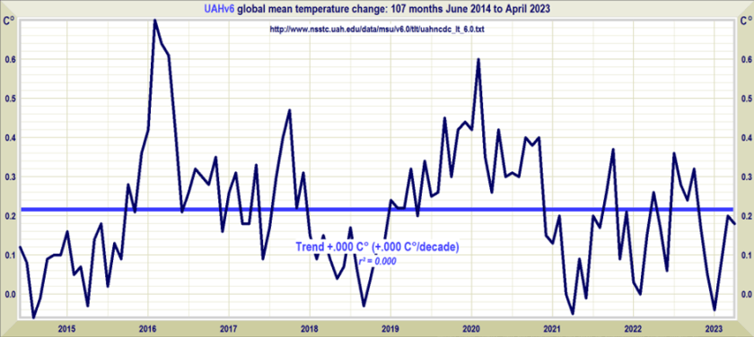
The New Pause has lengthened by a further two months to 8 years 11 months. The least-squares linear-regression trend on the UAH monthly satellite global-temperature dataset for the lower troposphere shows no global warming at all from June 2014 to April 2023.
As usual, the start and end dates of the New Pause are not cherry-picked. The end date is the most recent month for which data are available; the start date is the farthest back one can reach and still find a zero trend. It is what it is.
For comparison, here is the entire dataset for 44 years 5 months since December 1978. It shows a long-run warming rate equivalent to 1.3 K/century, of which 0.3 K has already occurred since January 2021, leaving just 1 K to go (on the current trend) until 2100, by which time reserves of coal, oil and gas will be largely exhausted.
We are no longer in la Niña conditions. They ended in March 2023, when the temperature of the Niño-3.4 region of the equatorial eastern Pacific rose above –0.5 K:
One reason why el Niño-watchers predict that an new el Niño is on its way is the gradual westward extension of the warm pool in in the top 300 m of the tropical Pacific, the hallmark of el Niño, as NOAA’s image shows –
NOAA thinks there is a 62% chance of an el Niño developing. If it does develop, it will probably bring the latest Pause to an end. Nevertheless, these long Pauses are a visual demonstration of the now-undeniable fact that the rate of global warming predicted by IPCC in 1990 has proven to be greatly in excess of the subsequent outturn.
First, note that the 0.136 K/decade trend in the 400 months (exactly a third of a century) since 1990 is barely above the 0.133 K/decade trend since 1978. Notwithstanding business-as-usual increases in emissions, very little acceleration in the global-warming rate is evident.
In fact, IPCC’s midrange prediction in 1990 of 0.3 K/decade business-as-usual warming since that year exceeds the 0.136 K/decade real-world global warming rate observed since then by a startling 120%. Indeed, even the 0.2 K/decade lower bound of IPCC’s 1990 prediction exceeds observed reality by close to half. Yet policy is being made by scientifically-illiterate governments on the basis of the 0.5 K/decade upper-bound prediction, which exceeds observed reality by a shocking 268%.
Annual emissions are indeed tracking the business-as-usual Scenario A in IPCC (1990). The growth is almost double that which was predicted under Scenario B. It is now clear that IPCC’s conversion of emissions to forcings, and thus its predictions of global warming, had been grossly overwrought and that, therefore, the threatened “climate emergency” is absent.
The Version 6 global average lower tropospheric temperature (LT) anomaly for April 2023 was +0.18 deg. C departure from the 1991-2020 mean. This is down slightly from the March 2023 anomaly of +0.20 deg. C.
The Version 6 global average lower tropospheric temperature (LT) anomaly for April 2023 was +0.18 deg. C departure from the 1991-2020 mean. This is down slightly from the March 2023 anomaly of +0.20 deg. C.
The linear warming trend since January, 1979 remains at +0.13 C/decade (+0.11 C/decade over the global-averaged oceans, and +0.18 C/decade over global-averaged land).
Various regional LT departures from the 30-year (1991-2020) average for the last 16 months are:
YEAR
MO
GLOBE
NHEM.
SHEM.
TROPIC
USA48
ARCTIC
AUST
2022
Jan
+0.03
+0.06
-0.00
-0.23
-0.13
+0.68
+0.10
2022
Feb
-0.00
+0.01
-0.01
-0.24
-0.04
-0.30
-0.50
2022
Mar
+0.15
+0.27
+0.03
-0.07
+0.22
+0.74
+0.02
2022
Apr
+0.26
+0.35
+0.18
-0.04
-0.26
+0.45
+0.61
2022
May
+0.17
+0.25
+0.10
+0.01
+0.59
+0.23
+0.20
2022
Jun
+0.06
+0.08
+0.05
-0.36
+0.46
+0.33
+0.11
2022
Jul
+0.36
+0.37
+0.35
+0.13
+0.84
+0.55
+0.65
2022
Aug
+0.28
+0.31
+0.24
-0.03
+0.60
+0.50
-0.00
2022
Sep
+0.24
+0.43
+0.06
+0.03
+0.88
+0.69
-0.28
2022
Oct
+0.32
+0.43
+0.21
+0.04
+0.16
+0.93
+0.04
2022
Nov
+0.17
+0.21
+0.13
-0.16
-0.51
+0.51
-0.56
2022
Dec
+0.05
+0.13
-0.03
-0.35
-0.21
+0.80
-0.38
2023
Jan
-0.04
+0.05
-0.14
-0.38
+0.12
-0.12
-0.50
2023
Feb
+0.08
+0.17
0.00
-0.11
+0.68
-0.24
-0.12
2023
Mar
+0.20
+0.23
+0.16
-0.14
-1.44
+0.17
+0.40
2023
Apr
+0.18
+0.11
+0.25
-0.03
-0.38
+0.53
+0.21
The full UAH Global Temperature Report, along with the LT global gridpoint anomaly image for April, 2023 should be available within the next several days here.
The global and regional monthly anomalies for the various atmospheric layers we monitor should be available in the next few days at the following locations:
Guest Essay by Dr. Alan Welch FBIS FRAS, Ledbury, UK — 3 May 2023
The release of the Sea Level Data up to Jan 2023 marks 30 years of satellite measurements using the quartet of satellites Topex and Jason 1, 2 and 3. It also marks 5 years of my interest in sea level rises, not as a climate scientist, but as a chartered engineer with nearly 40 years’ experience in engineering analysis. This interest was stimulated by the 2018 paper by Nerem et al (1) in which they introduced the concept of dangerously high sea level accelerations.
A year ago, I produced 2 essays. The first essay (2) showed the “accelerations” derived were probably the outcome of the methodology used. The second essay (3) showed that 30 years is too short a period to derive a meaningful acceleration.
The important graph in this update is Figure 3 which shows the change in “accelerations” using the Nerem approach when applied to the NASA data set and also to a sinusoidal data set. When accelerations are embedded in “ “ it implies these are based on 2 times the quadratic coefficient of a curve fit and may not necessarily be considered as a physical acceleration per se.
Every 1, 2 or 3 months the sea level data is released on the https://climate.nasa.gov/vital-signs/sea-level/ web site and these data have been analysed continuously since Feb 2018. The latest readings were downloaded via the April 2023 NASA Climate Change Newsletter. Figure 1 shows the NASA Data together with linear and quadratic best fit curves.
It is much easier to see trends when just the “Residuals”, the differences between actual values and the straight line, these being plotted in Figure 2.
For most of the analyses since 2018 a sinusoidal curve with a period of 22 years and an amplitude of +/- 3.5 mm was used. In reference 2 this was judged as needing updating and the period and amplitude were increased by about 20% and a small change in phase shift applied. The standard deviation of the residuals is 4.12mm whilst the standard deviations of the actual results about the quadratic and sinusoidal curves are 3.06 and 3.01 mm respectively implying that the sinusoidal may be a slightly better fit. (The use of an amplitude of +/- 4.2 mm is slightly embarrassing as it implies a degree of exactitude that many “climate scientists” would be proud of!).
In reference 2 the process of calculating “accelerations” for each successive batch of readings was applied to the sinusoidal curve and the resulting “acceleration” using the modified sinusoidal curve plotted in Figure 3 together with the actual derived “accelerations”. The sinusoidal curve has been (rightly or wrongly) extended to the year 2026. If extended much further the curve would approach zero in an oscillatory manner as shown in Note 2 of Reference 2 but this should not be considered a definite long-term prediction. The main danger in all climate change work is Extrapolation – a few years may be justified but many graphs are produced with eye watering amounts of extrapolation. Note the curve labelled “Sinusoidal” is not sinusoidal in shape but relates to the fact that it is based on the sinusoidal data. (In the comments in reference 2 the way the original sinusoidal curve was handled was justifiably criticised as not being mathematically precise, but a pragmatic engineering approach (aka gut feeling) led to the idea presented in figure 3. With the previous sinusoidal equation, the 2 curves were separated by 3 years but displayed sufficient similarity as to point to a promising line of enquiry).
The calculated “accelerations” have been reducing with every set of data since peaking in Jan 2020 and Figure 4 plots the % reduction in perceived “accelerations” since Jan 2020. This works out at about 4.5% reduction per year. On the NASA Web Site reference is made to the recent La Niña event having reduced the “acceleration” so it will be interesting to see what the next year or two will bring.
Figure 5 combines the Linear Fit with the Sinusoidal Variation.
Main Findings
1 The perceived “accelerations” have been reducing month on month since peaking in Jan 2020.
2 The Quadratic and Sinusoidal curves fit equally well. Remember they are products of the data available and great restraint must be used if extrapolation is contemplated.
3 Should the reduction in “accelerations” follow that shown by the sinusoidal curve as shown in figure 3 in 5 years’ time or so the “acceleration” should be down to nearly half the 2020 peak. (In 5 years, I’ll be over 90 so hopefully someone else will pick up the batten if I shuffle off this mortal coil!)
4 A question (hypothetical?) that could be asked is if there is a small sinusoidal content in the variations where does it come from? Possibly it is not within the data as measured but comes about by what is not measured. The satellite readings only cover about 95% of the oceans. If there are decadal ocean oscillations across the +/- 65 degree latitudes this could show up as a sinusoidal variation. Figure 6, from the NOAA site (https://www.star.nesdis.noaa.gov/socd/lsa/SeaLevelRise/LSA_SLR_timeseries.php) shows the extent of the ignored polar regions in relation to the polar seas.
5 The variation considered is only +/- 4.2 mm – that’s just over 0.16 inches in old money – which is next to nothing in comparison with some of the ocean variation given in the NOAA site over the last 30 years. Examples worth inspecting are the northerly seas such as the Bering Sea and the North Sea. Figure 7, taken from the University of Colorado site, https://sealevel.colorado.edu/data, showing variations of 20cm or more over the last 30 years. A change of 4.2 mm would only be as big as the “o” in Colorado!
Dr. Welch has been working on these analyses for years and has put his findings for the now-30-year climatic-period length of satellite era sea level measurements together in this essay. This and his two previous essays on the topic (linked in the essay and in the references) are offered here by Dr. Welch as an alternative hypothesis to Nerem (2018) ( .pdf ) and Nerem (2022). [ In a practical sense, Nerem (2022) did not change anything substantial from the 2018 paper previously discussed by Welch.]
I find Dr. Welch’s analyses interesting and feel strongly that Dr. Welch’s analyses deserve to be seen and discussed. I have encouraged him to present his findings here at WUWT.
Dr. Welch lives in the U.K. and his responses to comments on this essay will be occurring on British Summer Time : UTC +1.
The Contracts for Difference introduced by Ed Davey were poorly designed from the start, and are now costing energy users a fortune.
We already know that the contracts place no obligation whatsoever on generators to actually take up their options, enabling them to take advantage of much higher market prices as a result.
But just as costly has been the decision to index link strike prices each year for inflation. Given that most of the cost of a wind or solar farm is the capital cost, the indexation should only have applied to the operational cost.
This year’s price rise took effect at the beginning of April, and for offshore wind farms averages 11.9%. (For some reason I have not got to the bottom of, the increases vary slightly between generators).
This will cost energy users about an extra £360 million a year, based on last year’s outputs for all CfD generators. It puts the average cost of offshore wind up to about £175/MWh, compared to the current market price of around £100/MWh.
Since 2019, prices have risen by about 23%, costing consumers around £700 million a year now in total.
Lots of people support climate action – but that support wanes dramatically when the proposed actions are personally inconvenient, like giving up your automobile.
Many Europeans want climate action – but less so if it changes their lifestyle, shows poll
Exclusive: YouGov survey in seven countries tested backing for government and individual action on crisis
Many Europeans are alarmed by the climate crisis and would willingly take personal steps and back government policies to help combat it, a survey suggests – but the more a measure would change their lifestyle, the less they support it.
…
Measures entailing no great lifestyle sacrifice were popular, with between 45% (Germany) and 72% (Spain) backing government tree-planting programmes and 60% (Spain) and 77% (UK) saying they would grow more plants themselves or were doing so already.\
…
Even more radical proposals, such as voluntarily eating no more meat and dairy and having fewer children than you would like, were supported by between barely 10% (Germany) and 19% (Italy), and 9% (Germany) and 17% (Italy) respectively.
Changes in car use, a major contributor to carbon emissions and an area in which many European governments are already legislating, also drew responses that showed a close correlation to the impact they might have on people’s lives.
What a surprise – not. Personally I blame greens for this dissonance between people’s expectations and what greens think is required to save us from the carbon demon.
So why all this talk of personal sacrifice and lifestyle changes? If green is easier and cheaper, why should anyone need to make any sacrifices?
You can’t have it both ways greens. Either green is cheaper and better, which eliminates the need for significant personal sacrifice, or someone has been telling a few fibs.
This suggests that humans and the biosphere were enhanced by a warming process that has ended. The solar cycles are again going quiet and are forecast to continue that way.
Figure 1. Graph showing the number of volcanoes reported to have been active each year since 1800 CE. Total number of volcanoes with reported eruptions per year (thin upper black line) and 10-year running mean of same data (thick upper red line). Lower lines show only the annual number of volcanoes producing large eruptions (>= 0.1 km3 of tephra or magma) and scale is enlarged on the right axis; thick red lower line again shows 10-year running mean. Global Volcanism Project Discussion
Update April 28, 2023
I am prompted by a discussion at WUWT regarding the role of SO2 in causing climate variabiity. There are some voices claiming that reduced SO2 from smaller vocanic activity in the Middle Ages caused warming, leading to droughts, crop failures, etc. And that we could be causing global warming by removing SO2 from the air in modern times. As the research cited below explains, there is a likely role for volcanic SO2 to cause global cooling, which resulted in the crop failures and the “dark ages”.
In discussion with Kip Hansen, it occurred to me that the process and equation could be explained by the steady recovery from the LIA (Little Ice Age). That reminded me of this relevant discussion about the causes of the LIA, what ended it, and why the warming recovery from it may now be over.
Volcanoes and the Little Ice Age
University of Bern confirms in a recent announcement that volcanoes triggered the depths of the LIA (Little Ice Age). Their article is Volcanoes shaped the climate before humankind. H/T GWPF. However, they spin the story in support of climate alarm (emergency, whatever), rather than making the more obvious point that recent warming was recovering to roughly Medieval Warming levels after the abnormal cooling disruption from volcanoes. Excerpt in italics with my bolds.
“The new Bern study not only explains the global early 19th century climate, but it is also relevant for the present. “Given the large climatic changes seen in the early 19th century, it is difficult to define a pre-industrial climate,” explains lead author Stefan Brönnimann, “a notion to which all our climate targets refer.” And this has consequences for the climate targets set by policymakers, who want to limit global temperature increases to between 1.5 and 2 degrees Celsius at the most. Depending on the reference period, the climate has already warmed up much more significantly than assumed in climate discussions. The reason: Today’s climate is usually compared with a 1850-1900 reference period to quantify current warming. Seen in this light, the average global temperature has increased by 1 degree. “1850 to 1900 is certainly a good choice but compared to the first half of the 19th century, when it was significantly cooler due to frequent volcanic eruptions, the temperature increase is already around 1.2 degrees,” Stefan Brönnimann points out.”
Bern seems preoccupied with targets and accounting, while others are concerned to understand the role of volcanoes in natural climate change. A previous post gives a more detailed explanation, thanks to a suggestion I received.
The LIA Warming Rebound Is Over
Thanks to Dr. Francis Manns for drawing my attention to the role of Volcanoes as a climate factor, particularly related to the onset of the Little Ice Age (LIA), 1400 to 1900 AD. I was aware that the temperature record since about 1850 can be explained by a steady rise of 0.5C per century rebound overlaid with a quasi-60 year cycle, most likely oceanic driven. See below Dr. Syun Akasofu 2009 diagram from his paper Two Natural Components of Recent Warming.
When I presented this diagram to my warmist friends, they would respond, “But you don’t know what caused the LIA or what ended it!” To which I would say, “True, but we know it wasn’t due to burning fossil fuels.” Now I find there is a body of evidence suggesting what caused the LIA and why the temperature rebound may be over. Part of it is a familiar observation that the LIA coincided with a period when the sun was lacking sunspots, the Maunder Minimum, and later the Dalton.
Not to be overlooked is the climatic role of volcano activity inducing deep cooling patterns such as the LIA. Jihong Cole-Dai explains in a paper published 2010 entitled Volcanoes and climate. Excerpt in italics with my bolds.
There has been strong interest in the role of volcanism during the climatic episodes of Medieval Warm Period (MWP,800–1200 AD) and Little Ice Age (LIA, 1400–1900AD), when direct human influence on the climate was negligible. Several studies attempted to determine the influence of solar forcing and volcanic forcing and came to different conclusions: Crowley and colleagues suggested that increased frequency of stratospheric eruptions in the seventeenth century and again in the early nineteenth century was responsible in large part for LIA. Shindell et al. concluded that LIA is the result of reduced solar irradiance, as seen in the Maunder Minimum of sunspots, during the time period. Ice core records show that the number of large volcanic eruptions between 800 and 1100 AD is possibly small (Figure 1), when compared with the eruption frequency during LIA. Several researchers have proposed that more frequent large eruptions during the thirteenth century(Figure 1) contributed to the climatic transition from MWP to LIA, perhaps as a part of the global shift from a warmer to a colder climate regime. This suggests that the volcanic impact may be particularly significant during periods of climatic transitions.
Weighted annual average concentration of volcanic sulfate for the period of 176–2005 AD in a South Pole, Antarctica ice core (Cole-Dai, manuscript in preparation).
How volcanoes impact on the atmosphere and climate
The major component of volcanic eruptions is the matter that emerges as solid, lithic material or solidifies into large particles, which are referred to as ash or tephra. These particles fall out of the atmosphere very rapidly, on timescales of minutes to a few days, and thus have no climatic impacts but are of great interest to volcanologists, as seen in the rest of this encyclopedia. When an eruption column still laden with these hot particles descends down the slopes of a volcano, this pyroclastic flow can be deadly to those unlucky enough to be at the base of the volcano. The destruction of Pompeii and Herculaneum after the AD 79 Vesuvius eruption is the most famous example.
Volcanic eruptions typically also emit gases, with H2O, N2, and CO2 being the most abundant. Over the lifetime of the Earth, these gases have been the main source of the Earth’s atmosphere and ocean after the primitive atmosphere of hydrogen and helium was lost to space. The water has condensed into the oceans, the CO2 has been changed by plants into O2 or formed carbonates, which sink to the ocean bottom, and some of the C has turned into fossil fuels. Of course, we eat plants and animals, which eat the plants, we drink the water, and we breathe the oxygen, so each of us is made of volcanic emissions. The atmosphere is now mainly composed of N2 (78%) and O2 (21%), both of which had sources in volcanic emissions.
Of these abundant gases, both H2O and CO2 are important greenhouse gases, but their atmospheric concentrations are so large (even for CO2 at only 400 ppm in 2013) that individual eruptions have a negligible effect on their concentrations and do not directly impact the greenhouse effect. Global annually averaged emissions of CO2 from volcanic eruptions since 1750 have been at least 100 times smaller than those from human activities. Rather the most important climatic effect of explosive volcanic eruptions is through their emission of sulfur species to the stratosphere, mainly in the form of SO2, but possibly sometimes as H2S. These sulfur species react with H2O to form H2SO4 on a timescale of weeks, and the resulting sulfate aerosols produce the dominant radiative effect from volcanic eruptions.
The major effect of a volcanic eruption on the climate system is the effect of the stratospheric cloud on solar radiation (Figure 53.1). Some of the radiation is scattered back to space, increasing the planetary albedo and cooling the Earth’s atmosphere system. The sulfate aerosol particles (typical effective radius of 0.5 mm, about the same size as the wavelength of visible light) also forward scatter much of the solar radiation, reducing the direct solar beam but increasing the brightness of the sky. After the 1991 Pinatubo eruption, the sky around the sun appeared more white than blue because of this. After the El Chicho´n eruption of 1982 and the Pinatubo eruption of 1991, the direct radiation was significantly reduced, but the diffuse radiation was enhanced by almost as much. Nevertheless, the volcanic aerosol clouds reduced the total radiation received at the surface.
Although solar variability has often been considered the primary agent for LIA cooling, the most comprehensive test of this explanation (Hegerl et al., 2003) points instead to volcanism being substantially more important, explaining as much as 40% of the decadal-scale variance during the LIA. Yet, one problem that has continually plagued climate researchers is that the paleo-volcanic record, reconstructed from Antarctic and Greenland ice cores, cannot be well calibrated against the instrumental record. This is because the primary instrumental volcano reconstruction used by the climate community is that of Sato et al. (1993), which is relatively poorly constrained by observations prior to 1960 (especially in the southern hemisphere).
Here, we report on a new study that has successfully calibrated the Antarctic sulfate record of volcanism from the 1991 eruptions of Pinatubo (Philippines) and Hudson (Chile) against satellite aerosol optical depth (AOD) data (AOD is a measure of stratospheric transparency to incoming solar radiation). A total of 22 cores yield an area-weighted sulfate accumulation rate of 10.5 kg/km2 , which translates into a conversion rate for AOD of 0.011 AOD/ kg/km2 sulfate. We validated our time series by comparing a canonical growth and decay curve for eruptions for Krakatau (1883), the 1902 Caribbean eruptions (primarily Santa Maria), and the 1912 eruption of Novarupta/Katmai (Alaska)
We therefore applied the methodology to part of the LIA record that had some of the largest temperature changes over the last millennium.
Figure 2: Comparison of 30-90°N version of ice core reconstruction with Jones et al. (1998) temperature reconstruction over the interval 1630-1850. Vertical dashed lines denote levels of coincidence between eruptions and reconstructed cooling. AOD = Aerosol Optical Depth.
The ice core chronology of volcanoes is completely independent of the (primarily) tree ring based temperature reconstruction. The volcano reconstruction is deemed accurate to within 0 ± 1 years over this interval. There is a striking agreement between 16 eruptions and cooling events over the interval 1630-1850. Of particular note is the very large cooling in 1641-1642, due to the concatenation of sulfate plumes from two eruptions (one in Japan and one in the Philippines), and a string of eruptions starting in 1667 and culminating in a large tropical eruption in 1694 (tentatively attributed to Long Island, off New Guinea). This large tropical eruption (inferred from ice core sulfate peaks in both hemispheres) occurred almost exactly at the beginning of the coldest phase of the LIA in Europe and represents a strong argument against the implicit link of Late Maunder Minimum (1640-1710) cooling to solar irradiance changes.
Figure 1: Comparison of new ice core reconstruction with various instrumental-based reconstructions of stratospheric aerosol forcing. The asterisks refer to some modification to the instrumental data; for Sato et al. (1993) and the Lunar AOD, the asterisk refers to the background AOD being removed for the last 40 years. For Stothers (1996), it refers to the fact that instrumental observations for Krakatau (1883) and the 1902 Caribbean eruptions were only for the northern hemisphere. To obtain a global AOD for these estimates we used Stothers (1996) data for the northern hemisphere and our data for the southern hemisphere. The reconstruction for Agung eruption (1963) employed Stothers (1996) results from 90°N-30°S and the Antarctic ice core data for 30-90°S.
During the 18th century lull in eruptions, temperatures recovered somewhat but then cooled early in the 19th century. The sequence begins with a newly postulated unknown tropical eruption in midlate 1804, which deposited sulfate in both Greenland and Antarctica. Then, there are four well-documented eruptions—an unknown tropical eruption in 1809, Tambora (1815) and a second doublet tentatively attributed in part to Babuyan (Philippines) in 1831 and Cosiguina (Nicaragua) in 1835. These closely spaced eruptions are not only large but have a temporally extended effect on climate, due to the fact that they reoccur within the 10-year recovery timescale of the ocean mixed layer.
The ocean has not recovered from the first eruption so the second eruption drives the temperatures to an even lower state.
Abstract: Contrary to popular media and urban mythology the global warming we have experienced since the Little Ice Age is likely finished. A review of 10 temperature time series from US cities ranging from the hottest in Death Valley, CA, to possible the most isolated and remote at Key West, FL, show rebound from the Little Ice Age (which ended in the Alps by 1840) by 1870. The United States reached temperatures like modern temperatures (1950 – 2000) by about 1870, then declined precipitously principally caused by Krakatoa, and a series of other violent eruptions. Nine of these time series started when instrumental measurement was in its infancy and the world was cooled by volcanic dust and sulphate spewed into the atmosphere and distributed by the jet streams. These ten cities represent a sample of the millions of temperature measurements used in climate models. The average annual temperatures are useful because they account for seasonal fluctuations. In addition, time series from these cities are punctuated by El Nino Southern Oscillation (ENSO).
As should be expected, temperature at each city reacted differently to differing events. Several cities measured the effects of Krakatoa in 1883 while only Death Valley, CA and Berkeley CA sensed the minor new volcano Paricutin in Michoacán, Mexico. The Key West time series shows rapid rebound from the Little Ice Age as do Albany, NY, Harrisburg, PA, and Chicago. IL long before the petroleum-industrial revolution got into full swing. Recording at most sites started during a volcanic induced temperature minimum thus giving an impression of global warming to which industrial carbon dioxide is persuasively held responsible. Carbon dioxide, however, cannot be proven responsible for these temperatures. These and likely subsequent temperatures could be the result of regression to the normal equilibriumtemperatures of the earth (for now). If one were to remove the volcanic punctuation and El Nino Southern Oscillation (ENSO) input many would display very little alarming warming from 1815 to 2000. This review illustrates the weakness of linear regression as a measure of change. If there is a systemic reason for the global warming hypothesis, it is an anthropogenic error in both origin and termination. ENSO compliments and confirms the validity of NOAA temperature data. Temperatures since 2000 during the current hiatus are not available because NOAA has closed the public website.
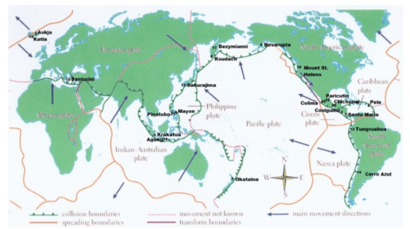
Example of time series from Manns. Numbers refer to major named volcano eruptions listed in his paper. For instance, #3 was Krakatoa
The cooling effect is said to have lasted for 5 years after Krakatoa erupted – from 1883 to 1888. Examination of these charts, However, shows that, e.g., Krakatoa did not add to the cooling effect from earlier eruptions of Cosaguina in 1835 and Askja in 1875. The temperature charts all show rapid rebound to equilibrium temperature for the region affected in a year or two at most.
Fourteen major volcanic eruptions, however, were recorded between 1883 and 1918 (Robock, 2000, and this essay). Some erupted for days or weeks and some were cataclysmic and shorter. The sum of all these eruptions from Krakatoa onward effected temperatures early in the instrumental age. Judging from wasting glaciers in the Alps, abrupt retreat began about 1860).
Manns Conclusions: 1) Four of these time series (Albany, Harrisburg, Chicago and Key West) show recovery to the range of today’s temperatures by 1870 before the eruption of Askja in 1875. The temperature rebounded very quickly after the Little Ice Age in the northern hemisphere.
2)Volcanic eruptions and unrelated huge swings shown from ENSO largely rule global temperature. Volcanic history and the El Nino Southern Oscillation (ENSO) trump all other increments of temperature that may be hidden in the lists.
3) The sum of the eruptions from Krakatoa (1883) to Katla (1918) and Cerro Azul (1932) was a cold start for climate models.
4) It is beyond doubt that academic and bureau climate models use data that was gathered when volcanic activity had depressed global temperature. The cluster from Krakatoa to Katla (1883 -1918) were global.
5) Modern events, Mount Saint Helens and Pinatubo, moreover, were a fraction of the event intensity of the late 19th and early 20th centuries eruptions.
6)The demise of frequent violent volcanos has allowed the planet to regress toward a norm (for now).
The forecast above did not mention the January 15, 2022 major eruption of Hunga Ha’apai volcano in Tonga.
Summary
These findings describe a natural process by which a series of volcanoes along with a period of quiet solar cycles ended the Medieval Warm Period (MWP), chilling the land and inducing deep oceanic cooling resulting in the Little Ice Age. With much less violent volcanic activity in the 20th century, coincidental with typically active solar cycles, a Modern Warm Period ensued with temperatures rebounding back to approximately the same as before the LIA.
This suggests that humans and the biosphere were enhanced by a warming process that has ended. The solar cycles are again going quiet and are forecast to continue that way. Presently, volcanic activity has been routine, showing no increase over the last 100 years. No one knows how long will last the current warm period, a benefit to us from the ocean recovering after the LIA. But future periods are as likely to be cooler than to be warmer compared to the present.
The United Kingdom is likely to have barely a quarter of the energy in 2050 promised by the Government and its Climate Change Committee if all the legal obligations of Net Zero are followed.
The United Kingdom is likely to have barely a quarter of the energy in 2050 promised by the Government and its Climate Change Committee if all the legal obligations of Net Zero are followed. This shocking news is forecast by the latest energy review recently published by U.K. FIRES. Government-funded U.K FIRES writes that the “whole excitement” of its project has been to recognise that such a shortfall is close to a certain reality. Excitement is not perhaps a word that comes immediately to mind when contemplating Britain’s almost certain economic and societal collapse.
As we have noted before in the Daily Sceptic, UK FIRES bases its recommendations on the brutal, and many would argue, honest reality of Net Zero. It does not assume that technological processes still to be perfected, or even invented, will somehow lead to minimal disturbance in comfortable industrialised lifestyles. Speaking to architects in 2021 at a RIBA climate conference, UK FIRES leader, Cambridge-based Professor Julian Allwood, said the UK Net Zero strategy is as unrealistic as “magic beans fertilised by unicorn’s blood”.
It can be argued that the £5 million of taxpayer funding to UK FIRES is money well spent since its honest Net Zero appraisals contrast with the fanciful stories and deceit that surround many other claims by Net Zero promoters.
The above graph shows how UK FIRES expects only one quarter of electrical power to be available in 2050, compared with all other forecasts. By 2050, electrical power will be the primary source of all energy. It notes that all other scenarios depend on negative emissions technologies such as carbon capture to deal with ‘residual emissions’ – shown in the graph in orange. UK FIRES notes that it reflects the reality that to date no such technologies are operating in the UK, and therefore it states that by 2050, “we should continue to anticipate that they would not exist”.
Allwood, and his colleagues from a number of universities including Oxford and Imperial College, are dismissive of many of the proposed Net Zero mitigation technologies, noting, for instance, that biofuels are unsustainable since they threaten biodiversity. In 2021, Allwood observed that delivering Net Zero by 2050 “will require governments to utilise all available abatement opportunities, yet current policy largely ignores socially-driven mitigation in favour of technological innovation in the energy sector”
In plainer English, these government driven social “abatement opportunities” might reference the World Economic Forum’s advice that you will eat bugs, own nothing, and, it need hardly be added, be happy. As we have previously reported, UK FIRES promotes a world with no flying and shipping by 2050, drastic cuts in home heating, bans on beef and lamb consumption, and a ruthless purge on traditional building materials such as bricks, glass, steel and cement, to be replaced with materials such as “rammed earth”.
The UK Government is committed to reducing emissions by 68% from 1990 to 2030. Most of the easy cuts have been made with a switch from coal to gas, and the offshoring of a great deal of British manufacturing capacity. But the easy cuts, and the ubiquitous virtue signalling that goes with them, have ended. To comply with legal requirements going forward a massive ramp up of green energy is required, and there is little evidence that it is occurring.
The above graph from Atkins ‘Engineering Net Zero’ is referenced by the UK FIRES energy report. It analyses the build rates required to deliver the energy infrastructure predicted by the Climate Change Committee. There has, of course, been some building of renewable power sources in the last ten years, – wind and solar taxpayer subsidies of £12 billion a year for providing about 5% of total energy needs, attests to that – but nothing to suggest the build can ramp up to the required levels to even try to keep society functioning. Allwood notes that the correct interpretation of this graph is that it isn’t going to happen. “There is no possibility of this level of energy infrastructure being built by 2035, and if anything approaching this rate of construction is to happen beyond then, the public financing commitment needs to be made right now, before the next election.”
Mainstream media is very keen on horrific climate stories, but UK FIRES predictions are more or less ignored – presumably on the grounds they are the wrong type of Net Zero scares. But UK FIRES seems keen to scare the horses, noting that in articulating and promoting what it calls “opportunities”, it is aiming to open up “a more credible pathway to delivering zero emissions in reality”.
Chris Morrison is the Daily Sceptic’s Environment Editor.
Unless we challenge this outrageous narrative, it is only a matter of time until some deep green politician advances a plan to “rescue” children from those unfit climate denier parents, by placing “predatory deniers” into the same legal category as pedophiles.
“… if parents do nothing, they fail their children …”
What makes a good parent? Is acting on climate change as important as love and bedtime stories?
Craig Stanbury, Monash University Published: May 2, 2023 6.00am AEST
What makes a good parent? Most would say a good parent loves and nurtures their child with the ultimate aim of helping them flourish – now and into the future. A good parent will feed their child, give them space to play and time to use their imagination, make sure they get an education and medical care, listen to their troubles, and teach them to one day be autonomous adults.
However, does being a good parent involve anything more than this?
In her book, Parenting on Earth, philosopher and mother Elizabeth Cripps argues that to do right by their kids, parents must also attempt to do something about the problems caused by climate change.
…
Cripps does not claim that it will be possible to do this all the time. (Climate action needs to be balanced against other duties involved in raising a child.) It may seem futile at times. But, if parents do nothing, they fail their children.
My children, and those of many prominent polluters and climate denialists, will probably live to be part of that grim winnowing – a world that the Alan Joneses and Andrew Bolts of the world have laboured so hard to create.
How should Australia’s parents deal with those who labour so joyously to create a world in which a large portion of humanity will perish? As I have become ever more furious at the polluters and denialists, I have come to understand they are threatening my children’s well-being as much as anyone who might seek to harm a child.
Flannery shies away from articulating the logical conclusion of his suggestion that “predatory” climate deniers are harming their own children and the children of others, but it seems pretty obvious where this is headed.
Unless we challenge this outrageous narrative, it is only a matter of time until some deep green politician advances a plan to “rescue” children from those unfit climate denier parents, by placing “predatory deniers” into the same legal category as pedophiles.
Claims that climate scientists ‘have never seen anything like it’ don’t tell us much as human lifetimes are short compared to Earth’s climate variations. There’s the story of the drained lake that reappeared – so clearly it was once there before any talk of ‘climate change’.
Claims that climate scientists ‘have never seen anything like it’ don’t tell us much as human lifetimes are short compared to Earth’s climate variations. There’s the story of the drained lake that reappeared – so clearly it was once there before any talk of ‘climate change’. – – – High in the California mountains, a ski resort sits buried under layers of snow and ice, says Sky News.
Residents of Mammoth Lakes fear for their lives, and livelihoods, after a winter of record snowfalls.
Wooden houses are blanketed under white powder, cars are buried beneath cement-like drifts, and roads are lined by colossal snow banks stretching up to 50ft tall.
Every so often a dagger-like slab of snow or ice will slide from a rooftop and shatter on the ground.
They’re used to a lot of snow in Mammoth Lakes. In fact, it’s vital for the economic survival of the town but nobody could have expected what happened this winter.
A series of so-called atmospheric rivers – narrow bands of moisture which carry precipitation from the Pacific Ocean over the west coast of the United States – hit California.
These storms have been unusual in their frequency and intensity following a decade of drought, transforming the Golden State into the sodden state.
In Mammoth, the snow fall was three times the historical average. When we visit, a month past the peak, the walls of snow are still as tall as two double decker buses in parts. . . . In California’s central valley, the snow-capped mountains, far in the distance, are a spectre of doom.
The near-record rainfall in California is already transforming the landscape here and that is before the big melt begins.
Corcoran is a town of 25,000 people and home to some of America’s most productive farmland, with an agricultural industry worth $2bn (£1.6bn). It is currently witnessing the remarkable rebirth of Tulare Lake, once the largest body of freshwater west of the Mississippi.
Tulare Lake was drained by farmers before completely disappearing by the mid-part of last century. But it is reappearing with a vengeance, already covering 30 square miles, an area roughly the size of Coventry, it looks like a vast inland sea. Experts predict that over the next couple of months it could grow to 200 square miles.
The flooding here happened too quickly for people to prepare and some workers have returned to the edge of the new lake with rowing boats to try and retrieve their drowned equipment. . . . At the lake’s shoreline, helicopters fly in sandbags and the army, in tractors, are helping shore up the levee to try to protect the city of Corcoran. This area has now been declared a disaster zone.
We are there when the state’s governor, Gavin Newsom, pays a visit. Over the past year he has toured wildfires, drought sites and now numerous areas in California that are underwater.
“There’s not a climate expert or a meteorologist that doesn’t say the following: “We’ve never seen this weather at this level of intensity and extreme”. That’s what is exacerbating the conditions that we’re experiencing,” he says.






You must be logged in to post a comment.