Fritz Vahrenholt: Climate policy makes citizens’ holiday trips more expensive

Today I am dealing with the increase in the price of air travel due to the climate policy of the German government as well as with a new population forecast that calls into question the climate scenarios of the Intergovernmental Panel on Climate Change for 2100.

From KlimaNachrichten

By KlimaNachrichten Redakteur

Monthly newsletter from Fritz Vahrenholt

Dear Ladies and Gentlemen, The unusually strong warming of global temperatures since 2023 will decrease slightly in October 2024. I dealt with the possible causes in my last newsletter. This month’s measurement results can no longer be compared with those of previous months, as the team led by Dr. Spencer from the University of Alabama has eliminated one of the measurement satellites from the calculation, which no longer provided reliable results. Since this error had already lasted for several months, the measurement results have been corrected accordingly. This leads to values that are about 0.1 degrees Celsius lower.

Today I am dealing with the increase in the price of air travel due to the climate policy of the German government as well as with a new population forecast that calls into question the climate scenarios of the Intergovernmental Panel on Climate Change for 2100.

The federal government is making air travel more expensive for citizens and damaging Germany as a business location

Carsten Spohr, the CEO of Lufthansa, burst his collar. In the Bild newspaper on 12.10.24 he spoke plainly: “I am very concerned about the connection of our business location. The extreme increase in government costs in air transport continues to lead to a shrinking supply. More and more airlines are avoiding German airports or cancelling important connections.”

One of his points of criticism: the increase in the aviation tax – also known as ticket tax – decided by the traffic light government – from 1.5.2024 from about €1.5 billion to €2 billion. The aviation tax was passed under Angela Merkel in 2011, when there was no CO2 tax for aviation. It should be melted down and ultimately eliminated altogether if aviation participates in the European CO2 emissions trading system.

And indeed, after the introduction of the European emissions trading system for aviation, it was practice for years to offset the costs from the CO2 certificates against the aviation tax. Therefore, there was no double burden on air traffic, because the aviation tax was reduced by the corresponding amount of CO2 certificates. Now, since 2024, the cost of CO2 certificates for air travel has been rising due to EU regulations.

For the 7.6 million tonnes of CO2 emitted by aircraft departing from Germany (except for long-haul travel), €125 million in 2024, €250 million in 2025 and €500 million in 2026 (at today’s price of €67/tCO2) will have to be raised. Because the reduction amount for the aviation tax therefore became larger and larger, Red-Green-Yellow abolished the offsetting on 1.5.2024. At the same time, it has even raised the aviation tax by 25%. So if you want to have a lasting impact on air traffic in Germany, then you are burdening air travel twice:

1. The offsetting of aviation tax and CO2 levy will be abolished

2. And in addition, the aviation tax will be raised from 1.5 billion to around 2 billion.

This money, which air travelers have to fork out, ends up in Mr. Habeck’s Climate and Transformation Fund, from which solar and wind power operators are subsidized if the price of electricity on the stock exchange does not yield enough revenue. And of course, those companies that embark on the dream journey into the hydrogen economy with Robert Habeck will also receive money from this pot. Keep this in mind if you have to pay €70.83 in aviation tax – i.e. ticket tax – on your next long-distance trip. One could have reacted like the conservative government in Sweden. It has taken the rising CO2 prices for aviation as an opportunity to completely abolish the aviation tax as of July 1, 2024.

And the next solo effort to save the world at the expense of air traffic is just around the corner. The EU has decided that 2% of “climate-neutral fuels”, so-called SAFs (Sustainable Air-Fuels), must be used from 2025, 6% from 2030 and 70% in 2050. There are two production methods for this. On the one hand, SAF fuel can be produced from biomass CO2-free. On the other hand, it can be produced at great expense on the basis of green hydrogen. For this purpose, hydrogen would have to be produced by electrolysis using solar and wind power and, in a second step, the hydrogen would have to be converted into kerosene with CO2 (Fischer-Tropsch synthesis). As there are still no plants to produce enough fuel from green hydrogen, the EU has only mandated the use of hydrogen-based fuel from 2030 onwards, with a share of 1.2%.

But the German government has already prescribed a quota of 0.5% for hydrogen-based SAF fuel for 2026. In the event of non-compliance, penalties are due.
Carsten Spohr rightly complains on behalf of Lufthansa that these fuels are not yet available in sufficient quantities: “We would need about half of Germany’s electricity to produce enough fuels”. And further: “I don’t think Mr. Habeck will give me that”

To bring green policy out of dreamland and into reality, I’ll do the math: The total kerosene consumption of German airlines (mainly Lufthansa and its subsidiaries) was 9,707,797 m³ of kerosene in 2023. This corresponds to an energy content of 86 billion kilowatt hours (86 TWh). According to the Federal Environment Agency, the energy efficiency of the production of kerosene by hydrogen electrolysis based on solar and wind power and subsequent synthesis of hydrogen with CO2 has an efficiency of 41%. (Source: Power to Liquid, Federal Environment Agency 2022, p. 16). According to this, 210 TWh of electricity are needed to generate Lufthansa kerosene. This is more than the total generation from photovoltaics and wind energy in Germany in 2023, which is 47% in relation to the total generation of 450 TWh in 2023.

So Carsten Spohr has calculated correctly. By the way, the cost would be 3 times as high as conventional kerosene. (60 €ct/l today). But the nightmare doesn’t end there. You could simply make SAF fuel from biofuel, for example from rapeseed oil or sunflower oil. However, the EU has prohibited this: it may only come from biogenic waste (!). Therefore, Lufthansa is currently buying up all the fry fat that the airline can get in order to be able to meet the quota.

In Germany, there are 200,000 tons of frying fat. If German airlines were to use all frying fat, they would account for about 2% of their total kerosene consumption. Achieving a quota of 6% in 2030 seems hardly achievable. You can literally hear the resounding laughter of the managers of China Airlines, Turkish Airlines or Emirates. Incidentally, this political folly took place with the votes of the CDU, SPD, Greens and FDP in the European Parliament. And then it was approved by the traffic light government.

But if you let the Greens do what they want, there are even greater follies. The red-green Hamburg Senate increased the airport fee for passengers by 15% next year (election year). Hardly anyone will notice an increase of 2.30 €, one will have thought, the citizens have no alternative. In addition, the Senate decided not to let the increase come into force until after the election in March. But the airlines reacted because the Senate had no idea about the low margins of the airlines.

If airlines only charge €20-30 per passenger, €2.30 is the last straw. Ryanair, Eurowings and Condor immediately announced that they would massively cut the offer from Hamburg and let their planes fly where they find more favorable conditions. As a result, passengers will have to pay higher prices next summer because of the lower offer, and the airport will have less revenue due to a lack of about 500,000 passengers.
The TAZ reacted to the withdrawal of the airlines: “It’s possible!” and “That’s a win for climate protection”

The decline in the world’s population calls into question the forecasts of the Intergovernmental Panel on Climate Change

At this point, I have often criticized the exaggerated alarmist scenarios of the Intergovernmental Panel on Climate Change (IPCC). Only with unrealistic CO2 emissions (tripling!) can temperature forecasts of a frightening 3-5 degrees Celsius for the year 2100 be calculated with the help of the controversial climate models (8.5 scenario, see graph below). The realistic development of CO2 emissions is shown in the following figure with the 4.5 scenario. Even the Intergovernmental Panel on Climate Change only assumes a temperature increase to a total of 2.7 degrees Celsius. We know about the inadequacy of climate models, which cannot reflect effects such as the increased direct solar radiation due to thinning clouds in recent years. But let’s assume for a moment that the IPCC model calculations are realistic. Even then, there is reason to revise the results significantly downwards.

Model 4.5 assumes a population development of the world with a peak of 10.13 billion people in 2080. Even in 2100, the world’s population is still expected to be 9.88 billion – 1.7 billion more people than today. (see next graph red curve). The latest estimates paint a completely different picture. The world-renowned population research institution of the University of Washington IHME assumes a peak of 9.7 in an upper estimate
billion people in 2064 (see graph blue curve). In a lower estimate (yellow curve), they assume a peak of around 9 billion people in 2054. This lower estimate is supported by demographic expert Jesus Fernandes-Villaverde of the University of Pennsylvania. In 2100, about 3.5 billion fewer people would live on earth than the IPCC assumes.

The cause of the population decline is the worldwide and, with a delay, also in Africa, declining number of children even below the conservation number of 2.1. This development will begin as early as 2030.

This has serious consequences for CO2 emissions: fewer people – fewer CO2 emissions. Roger Pielke, former professor at the University of Boulder, Colorado, has calculated the consequences in his blog and comes to a 0.6 degree Celsius lower warming in 2100 in the IPCC models, namely 2.07 degrees. This would then be a warming that is at the upper end of the goals of the Paris Climate Agreement ( Article 2 : “the increase in the average global temperature is kept well below 2 °C above pre-industrial levels and efforts are made to limit the temperature increase to 1.5 °C above pre-industrial levels”)

Wouldn’t that be good news for the delegates of the 29th World Climate Change Conference, which will take place in Baku from 11 to 24 November? Compliance with the Paris climate target is therefore very likely if we continue on the very likely path of emissions development, namely a slight increase in emissions by 2050 and a gradual increase thereafter.
Reduction to about half of emissions by 2100. This would be achievable without a loss of prosperity. Which climate researcher dares to bring these realities to the attention of the federal government and thus correct its course of destroying the economic foundations of this country?

If science does not do it, citizens must do it and elect politicians who stop scaring citizens, who stop bullying citizens and companies into a CO2-free policy, who start giving back to citizens what they deserve: freedom, prosperity and a good future.

Sincerely
Your

Fritz Vahrenholt

Fossil Fuel Political Backfire (AEI’s Teixeira explains)

In his Free Press article “How Progressives Blew It,” Ruy Teixeira of the American Enterprise Institute, explained how the anti-fossil-fuel narrative of the Left backfired.

“Telling people fossil fuels are evil and they must stop using them was a terrible idea, and voters hate it,” he began.

From Master Resource

By Robert Bradley Jr.

In his Free Press article “How Progressives Blew It,” Ruy Teixeira of the American Enterprise Institute, explained how the anti-fossil-fuel narrative of the Left backfired.

“Telling people fossil fuels are evil and they must stop using them was a terrible idea, and voters hate it,” he began. 

Since the days of Barack Obama and an “all of the above” approach to energy production, progressives have embraced a radical approach to energy issues. They promulgated the view that climate change is not gradually advancing, but is already a crisis evident in extreme weather events. It threatens the existence of the planet without immediate, drastic action. That action must include the immediate replacement of fossil fuels by renewables, which are cheap and can be introduced right now with sufficient resources. 

Teixeira explained:

According to the progressive view, people resist rapidly eliminating fossil fuels only because of propaganda from the fossil fuel industry. Potential problems with renewables, such as their intermittency, are being solved, they argue. This means that as we use more renewables and cut out fossil fuels, political support for the transition to clean energy should rise because of the benefits to consumers, who will have cheaper energy costs, and to workers, who will have high-paying clean energy jobs.

False assumptions and snobbery have not impressed the electorate, the opposite being the case.

This is the gospel for progressives who see themselves as noble warriors against the impending apocalypse. But most voters, especially working-class voters, have not signed up for—or are even much interested in—the rapid green transition they envision.

Too much, too fast–but Teixeira falls into the every-energy-in-the-stew approach, a governmental one.

Workers far prefer a gradual “all-of-the-above” approach to transitioning the energy system over the frantic push for renewables that characterizes progressives’ Green New Deal–type thinking. In our Politics Without Winners survey, we asked respondents whether they thought the country’s energy supply should “use a mix of energy sources including oil, coal, and natural gas along with renewable energy sources,” or “phase out the use of oil, coal, and natural gas completely, relying instead on renewable energy sources such as wind and solar power only.” An overwhelming 72 percent in the survey favored the all-of-the-above approach, while just 26 percent backed the rapid renewables transition. Views were even more lopsided among working-class voters.

He continues:

The hard fact is that progressives’ hostility to fossil fuels is not widely shared by ordinary voters. In a recent result from a New York Times/Siena College poll, two-thirds of likely voters said they supported a policy of “increasing domestic production of fossil fuels such as oil and gas.”  Two-thirds!

Home-grown exportable energy, what Trump calls ‘liquid gold’, has voter standing.

A new NBC poll tested a wide range of policy proposals to see whether voters would be more or less likely to support a candidate who espoused them. The single most positive response among voters was to a proposal to expand domestic oil and natural gas production. By a very wide 67 to 15 percent margin, voters said they would be more likely to support a candidate who wanted to expand fossil fuel production.

“Voters clearly aren’t buying what progressives are selling on energy and climate,” Ruy Teixeira concludes. “Not even close. And that’s another big reason the progressive moment has come to an end.”

We are left with Kamala Harris “furiously backpedaling from all these [anti-energy] positions,” but change takes time. Energy exceptionalism led by oil, gas, and coal is getting back in the saddle, even politically correct.

Miliband Lies About NESO Report

“Clean Power” is not achievable when you need a full fleet of gas power stations in reserve, to use when the wind does not blow!

From NOT A LOT OF PEOPLE KNOW THAT

By Paul Homewood

Ed Miliband has been caught out making two big fat lies:

“Clean Power” is not achievable when you need a full fleet of gas power stations in reserve, to use when the wind does not blow!

And electricity won’t be cheaper, even if you count Carbon Costs:

Natural Climate Change Factors

“Consensus” scientists do not believe that solar variability, internal climate variability (in this model simplified to the ~67-year stadium wave), or volcanism influence net global warming or climate change since 1750, yet considerable evidence exists that these factors have an impact. I’ve previously built a model of the HadCRUT5 global average temperature (see here) from seven known climate and solar cycles using multiple regression and was reasonably successful.

From Watts Up With That?

By Andy May

“Consensus” scientists do not believe that solar variability, internal climate variability (in this model simplified to the ~67-year stadium wave), or volcanism influence net global warming or climate change since 1750, yet considerable evidence exists that these factors have an impact. I’ve previously built a model of the HadCRUT5 global average temperature (see here) from seven known climate and solar cycles using multiple regression and was reasonably successful.

In this attempt, I utilize the six best documented solar/climate cycles in listed Table 1 and the stadium wave climate-only interior variability cycle to create a multiple regression model of HadCRUT5.

Table 1. Solar and climate proxies and measurements used in this model.

When using many series to build a multiple regression model one is always confronted with von Neuman’s joke that with four arbitrary parameters he can fit an elephant. Further, all these series are serially correlated, which weakens the computed statistics of the resulting fit, such as R2. However, none of these series are “arbitrary parameters.” Except for the stadium wave and Log2_CO2 they are observed solar and climate cycles that share the same period and are in phase with one another. All are well supported with multiple lines of evidence. Thus, they are quite constrained and not arbitrary.

While they are not arbitrary in the von Neuman sense, they are not independent of one another. Probably the solar dynamo is behind all of them, but the mechanism Sun → climate is not understood for any of them except possibly for the Hale Cycle and the Barycenter. The solar dynamo is quite complex, especially in the longer term.

The stadium wave has no associated solar cycle and seems to be wholly internal variability, it has a period of roughly 67 years and correlates well with global average temperature (May & Crok, 2024). Internal climate variability is poorly understood and simply choosing the stadium wave to represent it is probably a vast oversimplification, but it is the best I can do. For a good up-to-date discussion of the components of internal variability I recommend Marcia Wyatt’s excellent report on circulation patterns (Wyatt M. , Circulation Patterns: Atmospheric and Oceanic, 2020). The report is paywalled, but a slightly different earlier version of the same report can be downloaded here.

The whole point of including the stadium wave is to account for the variable lag in emitting received solar radiation to space. Most solar radiation is received in the tropics, more than they can emit to space. As a result, some of the radiation received in the tropics must be transported to higher latitudes which emit more energy than they receive, especially in the winter months. Atmospheric and ocean circulation patterns change the timing of this tropics-to-pole energy transfer. A longer time to emit absorbed solar energy causes the planet to warm and a shorter time causes it to cool. Earth is never in thermal equilibrium except briefly by coincidence and the thermal energy residence time in the ocean/atmosphere climate system is constantly changing but seems to have roughly a 67-year cycle. The 67-year cycle overlies a longer secular trend of change, that longer trend could be due to solar cycles or CO2 or both. See figure 2 in May & Crok as an example.

There are no measurements from space or in the atmosphere that support the hypothesis that additional CO2 (man-made or otherwise) will cause global warming, but there are lab measurements, correlations, and climate models that support the hypothesis. CO2 has some effect, but how much is anyone’s guess at this point. We try and use multiple regression to derive a value below.

Critical Solar and Cycles

In this section we briefly describe each of the six well documented solar cycles listed in Table 1 that have a demonstrated impact on Earth’s climate and provide references for them.

Bray/Hallstatt Cycle

Roger Bray used glacial advance and retreat records to identify an approximately 2400-year climate cycle originally called the “Hallstatt” cycle (Bray, 1968). Although originally discovered by its effect on Earth’s climate there is an associated solar cycle that is in phase with the climate cycle and has the same period as discussed here. A more technical discussion of the solar Bray/Hallstatt Cycle is presented by Ilya Usoskin et al. here (Usoskin, Gallet, Lopes, Kovaltsov, & Hulot, 2016). A low in the Bray Cycle played a role in creating the very cold period from about 1650-1715AD during the Little Ice Age.

Eddy Cycle

The roughly 1000-year Eddy Cycle was named by José A. Abreu and colleagues (Abreu, Beer, & Ferriz-Mas, 2010). They note that John Eddy identified and documented periods of very low solar activity that corresponded with colder climates on Earth, like the Little Ice Age (Eddy, 1976). The 1000-year climate cycle can be seen by combining the Medieval Warm Period (roughly 800 to 1250AD with the Little Ice Age (roughly 1300-1850AD). Solar proxies find a 1000-year solar cycle that is in phase with the climate cycle as pointed out by John Eddy, see figure 5 in (Eddy, 1976). More on the Eddy Cycle can be seen in Javier Vinós’ book (Vinós, 2022), Chapter 8, page 123 here. The powerful Bray Cycle and the Eddy Cycle both had lows between 1470 and 1680 which undoubtably contributed to that extremely cold time during the Little Ice Age. For more on the Little Ice Age see (May & Crok, 2024) and here.

De Vries Cycle

The De Vries Cycle is also often called the Suess Cycle after Hans Suess (Suess, 1955) and (Sonett & Suess, 1984). Like most cycles it was first discovered in climate proxies, especially tree ring records, and it has a period of 193-209 years. The matching solar cycle is probably related to a beat period between the fundamental Hale Solar Cycle and the rosette-like motion of the Sun around the solar system barycenter (Stefani, Horstmann, Klevs, Mamatsashvili, & Weier, 2023).

Feynman Cycle

It was always recognized that some sort of solar cycle existed with a period between 50 and 150 years and the mysterious poorly defined cycle was usually called the Gleissberg Cycle. Meanwhile a climate cycle with a length of about 100 years was also observed. Eventually Joan Feynman nailed down what is now called the ~100-year Feynman Solar Cycle in 2014 (Vinós, 2022, p. 129) and (Feynman & Ruzmaikin, 2014). We use a period of 105 years for the Feynman Cycle. The Feynman climate and solar cycles have the same period and are in phase.

Hale Cycle

The 22.14-year Hale Cycle is a very prominent solar cycle that is formed by a 22-year fundamental period of solar magnetic activity. It encapsulates two solar cycles that are marked by reversals of the solar magnetic field. Thus, one Hale cycle sees a reversal of the magnetic field and then a return to the original polarity. The Hale Cycle is closely related to the 22-year southwestern U.S. drought cycle (Mitchell, Stockton, & Meko, 1979).

Solar Barycenter rosette

The Sun tracks a complicated rosette-like motion about the solar system barycenter that takes 19.86 years (Stefani, Horstmann, Klevs, Mamatsashvili, & Weier, 2023). Any climate cycle associated with this is buried, or possibly shared, with the Hale Cycle.

Other Natural Climate Cycles

Stadium Wave

What we call the Stadium Wave Cycle or oscillation is a very strong global climate cycle that has a period of about 67 years (Wyatt & Curry, Role for Eurasian Arctic shelf sea ice in a secularly varying hemispheric climate signal during the 20th century, 2014) and (Wyatt M. G., 2012c). It is composed of many climate oscillations that propagate in an organized fashion across the Northern Hemisphere and affect the climate of much of the globe. It is not clear if this oscillation is related to a solar cycle.

CO2

CO2 as a factor that influences climate was first properly described by Svante Arrhenius in his book Worlds in the Making (Arrhenius S. , 1908), but he also discusses it in an earlier paper (Arrhenius S. , 1896). Even before Arrhenius’ attempt to quantify the atmospheric CO2 concentration’s impact on the climate, the idea that CO2 can affect Earth’s climate was also discussed, although in a less quantitative way, by Fourier (Fourier, 1824), Tyndall (Tyndall J. , 1861) and (Tyndall J. , 1859), and Langley (Langley, 1884). None of these earlier writers suggested that atmospheric CO2 concentration “controlled the climate,” as the IPCC proposes in AR6 and previous reports (IPCC, 2021, p. 179), (Lacis, Hansen, Russell, Oinas, & Jonas, 2013), and (Lacis, Schmidt, Rind, & Ruedy, 2010). They also did not believe that human CO2 and other greenhouse gas emissions were responsible for almost all the warming Earth has experienced since 1750 as claimed by the IPCC in AR6, page 961, figure 7.7.

None-the-less, CO2 and other greenhouse gas concentrations probably do influence the average atmospheric temperature, however the idea that they somehow “control” the global average surface temperature and climate change is highly doubtful.

Figure 1 is a plot of all the series discussed in this post.

Figure 1. The time series discussed in this post.

Discussion

If we use the top seven series listed in table one, that is everything but CO2, and regress against HadCRUT5 we get the result shown in orange in figure 2. If we then regress everything, including CO2, we get the blue dashed line in figure 2. The two lines are nearly identical.

Figure 2. The faint gray line is HadCRUT5, the orange line is a regression against it using only the solar and climate cycles, the blue dashed line uses the same cycles, but adds the Log, base 2, of CO2.

Now, that is interesting! The fit with the climate/solar cycles only and the fit with CO2 and the same cycles are nearly identical. We need more information to make sense of this. Below are the statistics of the two regressions.

Table 2. Statistics of the regression with all the solar/climate cycles, but no CO2. Adjusted R2 = 0.8523.

Table 2 shows the statistics of the regression with no CO2. The derived coefficients are on the left, and the mean and standard deviation of each series are shown and then the normalized coefficients. We can see that the Bray and Eddy Cycles are the most important series, and they slightly oppose one another since they have different signs. All the “P” values are good. The standard errors for the Bray and Eddy Cycles are a bit high, but that may be because their coefficients have opposite signs.

In Table 3 we show the statistics for the regression that contains CO2.

Table 3. The regression statistics when CO2 is added. Adjusted R2 = 0.8548

Table 3 contains a lot of new and valuable information. In Table 2 the normalized coefficients show that the Bray and Eddy Cycles dominated the regression, but in Table 3 it is CO2, by a long way and the P values for both Bray and Eddy have become unacceptable. CO2 has essentially replaced the strong Bray and Eddy Cycles and knocked them out. Removing those two cycles results in the De Vries cycle becoming unacceptable with a P value of 0.37, so I also removed it, and the result is shown in Table 4.

Table 4. The regression statistics when CO2 is added. Adjusted R2 = 0.8548

In Table 4 all the P values are acceptable and CO2 dominates the regression. For all practical purposes the adjusted R2 from all three regressions are identical at about 0.85. The “adjusted R2” is corrected for the number of predictor variables and the number of observations. In all these cases the regular R2 is nearly identical to the adjusted R2.

Figure 3 compares the no CO2 case to the case described in Table 4.

Figure 3. Comparing the all-cycles/no CO2 regression in blue to the CO2 and no Bray, Eddy or de Vries cycles in orange. Statistics for the orange regression are given in Table 4.

Conclusions

As usual in climate science (and statistical analysis) you can take away whatever you like from this analysis. Statistics and climate science are similar in this way, you can always generate a lot of discussion around either of them and still know nothing.

CO2 makes no difference if all the climate/solar cycles are used, but CO2 can replace the most powerful Bray, Eddy, and de Vries solar/climate cycles. Objectively, one could point out that solar cycles (including the Milankovitch cycles) have driven climate change as far back as we can trace them with proxies and historical records, so why would we think CO2 is driving climate if adding it to the regression makes no difference?

On the other hand, CO2 can replace the very powerful Bray, Eddy, and de Vries cycles and get the same result. As usual, this analysis just shows we have no clue what drives climate change, but isn’t that what we’ve been saying all this time?

One can look at these plots and statistics and conclude that the impact of CO2 on climate is zero, or they can conclude it is 100%. This study is inconclusive by itself. However, it also shows that well-known solar cycles, combined with internal variability can explain recent global warming; CO2 is not required to explain it.

As with all purely statistical studies, this regression model is unsuitable to use in forecasting or hindcasting, the large coefficients in tables 2 to 4 show that. The value of the study is only to demonstrate that CO2 is not necessary to explain recent warming.

This post looks at the problem “does CO2 control global warming?” from a statistical perspective. To see how experts in climate science look at it from an atmospheric physics perspective it is worth reviewing the excellent 2014 American Physical Society workshop on climate change hosted by Steve Koonin. It is discussed and summarized here.

This post is the result of many email conversations with Charlie May, who contributed substantially to the ideas and models presented herein.

Download the bibliography here

Download the Regression statistics here.

Download the data used and the plots here.

NESO Say We Must Keep All Our Gas Plants Going

According to NESO, most of this demand flexibility will revolve around smart charging of EVs and use of thermal storage. The idea of making us charge our EVs at night is hardly new; nor are electric storage heaters. But these only switch demand from one time of day to another, so are not really relevant in overall terms.

From NOT A LOT OF PEOPLE KNOW THAT

By Paul Homewood

h/t Philip Bratby

Well, the report into the feasibility of 2030 net zero targets from the electricity system operator, NESO, requested by Ed Miliband, has landed on his desk:

Millions more households could be asked to regularly switch off light and appliances under Ed Miliband’s plan for a clean power grid by 2030, an official review has found.

The Energy Secretary has been told that the Government’s pledge to rely on wind and solar farms for most of Britain’s power needs is technically achievable but will entail a “Herculean effort” on every front.

Advice published by the National Energy System Operator (Neso) said a quadrupling of so-called flexibility is needed in order to ensure the grid can operate without the use of fossil fuels.

https://www.telegraph.co.uk/business/2024/11/05/millions-more-switch-off-ed-miliband-net-zero-targets

The Telegraph, however, seems to have largely missed the point! (Not for the first time!)

In reality, Fintan Slye’s report is a bit of a damp squib, little more than a rehash of the Future Energy Scenarios. The plan can be downloaded here.

Let’s first deal with the issue of “switching off the lights”.

According to NESO, most of this demand flexibility will revolve around smart charging of EVs and use of thermal storage. The idea of making us charge our EVs at night is hardly new; nor are electric storage heaters. But these only switch demand from one time of day to another, so are not really relevant in overall terms.

Meanwhile, “turning the lights off” is planned to save only 3 GW – again a bit of a side issue. Residential electricity demand, by the way, peaks at around 15 GW in winter, so they would be looking at 1-in-5 households switching off. Good luck with that!

The real importance of this energy rationing, however, is that a decarbonised power grid cannot simply turn up the gas plants to match demand as it goes up and down during the day. What happens when we refuse to cooperate is another matter!

None of that addresses the problem though of what we will do when we get a week like this with virtually no wind power.

So what does the report actually say?

It reiterates existing Labour plans to double onshore wind power by 2030, triple offshore to 50 GW and triple solar as well.

Battery storage will quadruple to 22 GW, but as the report admits this is a drop in the ocean in terms of GWh. Same story with pumped storage. Their role will remain the same as now – maintaining grid frequency and topping up supply at peak periods.

So what will they do when the wind does not blow?

They have an answer – fire up the gas plants!

Indeed it would appear they need more than we currently have, around 35 GW they reckon:

So all of the bluster about 100% clean energy was a lie, as we have been saying all along. It is simply impossible to run a grid largely on intermittent renewables. Miliband’s plans were fantasy all along.

Sure, eventually they might replace all of this gas capacity with new gas plants fitted with carbon capture, or hydrogen burning plant using gas as a feed stock. But we will still be dependent on fossil fuels either way.

And keeping all of our gas capacity going for many more years to come brings with it its own problems:

You have to keep the plants fully manned all year, and you have to keep them well maintained. This all costs money. When owners of CCGT plants find they are only operational for a few days a year, what incentive will they have to keep them open. They will need billions of subsidies via the Capacity Market Mechanism to persuade, and probably a long term guarantee as well.

Which brings us to their assessment of costs.

They claim that all of this renewable generation will reduce generating costs by £15/MWh. But this is an outright lie, because they have included Carbon Costs in the cost of CCGT:

This is plainly absurd, a choice of being burnt or scalded. They have included £60/MWh in the cost of gas generation for carbon costs, meaning that instead of being £15/MWh cheaper, their plan would increase the cost of generation by about £10/MWh. (Allowing for the fact that not all dispatchable power comes from gas). But carbon costs are not real costs, and we would not need to buy permits if the government changed the way the Scheme works.

Add that to the indirect extra costs they mention, and we are looking at an extra cost of £35/MWh over the grid as a whole. That equates to a total annual cost of around £14 billion, on top of the £12 billion or so which we are already paying for renewables.

These costs do not include standby payments to gas generators, as mentioned above. These alone will run into several billions a year.

To cope with the huge rise in renewable capacity and increased demand for electricity, they say we will need to spend £14 billion a year on upgrading the grid till 2030. On top of that will come an extra £34 billion for building renewable capacity:

And all of this expenditure will merely end up duplicating what we already have. Where on Earth is the sense in that?

Right, Our World In Data, Climate Change Is Increasing Crop Yields, Concern About Future Decline Is Unwarranted

Our World In Data (OWID) ran a series of articles by Hannah Ritchie which explores the impact of climate change on crop production. On balance the stories get the facts straight, pointing out that yields of key staple crops have increased dramatically, in large part due to the CO2 fertilization effect and modestly warmer temperatures; however, parts of the stories stray into speculation that some crops have increased less than they would have and that they will decline in the future because of climate change. The latter claims are mistaken, based on disputed computer model outputs and unjustified beliefs about crop responses to modest temperature increases, not experience or data, which is what OWID should stick to.

From ClimateRealism

By H. Sterling Burnett

Our World In Data (OWID) ran a series of articles by Hannah Ritchie which explores the impact of climate change on crop production. On balance the stories get the facts straight, pointing out that yields of key staple crops have increased dramatically, in large part due to the CO2 fertilization effect and modestly warmer temperatures; however, parts of the stories stray into speculation that some crops have increased less than they would have and that they will decline in the future because of climate change. The latter claims are mistaken, based on disputed computer model outputs and unjustified beliefs about crop responses to modest temperature increases, not experience or data, which is what OWID should stick to.

Ritchie’s series of articles, “Crop yields have increased dramatically in recent decades, but crops like maize would have improved more without climate change,” “How will climate change affect crop yields in the future?,” and “Climate change will affect food production, but here are the things we can do to adapt,” are by and large well written, data driven pieces describing the current beneficial impact of climate change on crop production, and the tremendous potential of wider penetration of modern agricultural technologies into developing countries to increase production further. The only flaws in the articles are where she cites unverified studies depending upon flawed climate model projections to speculate concerning what might have happened to some crops absent warmer temperatures, and what might happen in the future.

Ritchie’s series starts off on solid ground noting the tremendous growth in cereal crops and regionally important staple crops. Ritchie writes:

When considering the net impacts of climate on food production, we need to consider three key factors: higher concentrations of CO2, warmer temperatures, and changes in rainfall (which can cause too much, or not enough, water).

…

Carbon dioxide helps plants grow in two ways.

First, it increases the rate of photosynthesis. Plants use sunlight to create sugars out of CO2 and water. When there’s more CO2 in the atmosphere, this process can go faster.

…

Second, it means plants can use water more efficiently

Ritchie then goes on to detail how higher CO2 concentrations have boosted crop yields. This is a fact that Climate Realism has pointed out in across more than 200 articles previously, here, here, and here to point to a few examples. Data from the U.N. Food and Agriculture Organization (FAO) show that wheat, rice, corn and other top cereal crops have repeatedly set new records for yield and production during the recent period of modest warming.

  • Cereal yields have increased nearly 52 percent, with the most recent record for yield set in 2022; and
  • Cereal production grew by approximately 57 percent. (see the chart, below)

There are three cereal crops Ritche expresses concern about, maize, millet, and sorghum, claiming that they would have increased more absent climate change, but that is based on a counterfactual analysis based on computer model projections, not data. She cites studies which suggest that many of the areas these crops are grown in have surpassed or are soon to surpass their optimal growing temperatures, with every increase above the maximum optimum range resulting in declining yields. Yet in the face of a 1.3℃ to 1.5℃ rise over the past century, all three of those crops have experienced substantial yield increases across recent decades, both globally and in the tropical developing Asian and African countries she worries might not be fully benefitting from CO2 fertilization.

Concerning maize, FAO data show that between 1991 and 2022, global maize yields increased by approximately 55 percent and about 49 percent in Africa.

The data from the FAO for millet and sorghum are similar, with each crop experiencing substantial yield gains, globally, and across Africa and Asia over the past three decades of modest warming. (see the graph below).

As has been discussed in more than 200 articles on Climate Realism, what is true of global cereal production, is true for most crops, like fruits, legumes, tubers, and vegetables, in most countries around the world. Yields have set records repeatedly during the recent period of climate change, food security has increased, and hunger and malnutrition have fallen.

Ritchie cites a few studies which suggest that the yields of maize, millet, and sorghum would have been even higher absent warming, which resulted in much of their growing regions experiencing temperatures outside of their optimal range — a problem which will only grow in the future if CO2 emissions aren’t restrained — but such claims suffer from a number of flaws. First, most of the regions of concern for the growth of maize, millet, and sorghum, sit astride or are near the equator. Yet the climate change theory says equatorial regions are least likely to experience much temperature rise – rather temperatures are expected to increase dramatically nearest the poles. Little or no temperature rise for the regions of concern means exceeding what some scientists speculate are optimum temperatures should not be a problem.

Second, Ritchie is right that changes in precipitation can reduce crop production, but once again, that should not be a concern. Many of the areas Ritchie highlights in Africa and Asia experience periodic or even seasonal drought. Since, as Ritchie notes, CO2 fertilization results in crops using water more efficiently, losing less water due to transpiration, crops should benefit. On the other hand, many countries in Africa and Asia depend on rainfall for crop production, with limited access to modern irrigation infrastructure. Here, climate change helps because most research suggests, and the IPCC projects, that climate change will result in increased precipitation, which means more water for crops, and if the water is seasonal as it is in many countries, more water that can be stored for use when rain or snowfall is lacking.

Third, the claim that climate change harms crops is contradictory in theory. Climate alarmists claim higher CO2 is driving rising temperatures – if so, the higher temperatures are a by-product of rising CO2, meaning without the CO2, temperatures might not rise. Yet, CO2 is the key factor driving growing crop yields, so absent increasing CO2, crops yields would have increased and continue to grow more slowly than they did, if at all. On this theory, if you want benefits CO2 fertilization, you have to accept the modest temperature increase. Cutting CO2 concentrations to avoid a minimal temperature rise would be to kill the golden goose for crop yields, resulting in a larger decline in or slower growth of yields than any modest decrease in yields that might result from the associated supposed small temperature rise.

What are we left with. Crop yields have increased due to rising CO2 concentrations, reducing hunger in the process. In addition, there is no reason to believe CO2 fertilization won’t continue to produce yield increased for the foreseeable future, unless climate policies result in lower CO2 concentrations.

On the other hand, as Ritchie points, out any foreseeable negative climate change impacts on crops, most especially in developing countries, would be far outweighed if they gain broader access to modern agricultural technologies, such as fertilizers, pesticides, modern farm equipment, and infrastructure. As Ritchie writes:

[T]here are other things we can do to mitigate this risk and counteract some of these pressures.

There are still huge yield gaps across the world today. “Yield gaps” are the difference between the yields that farmers currently get and could get if they had access to the best seeds, fertilizers, pesticides, irrigation, and practices that already exist today.

Let’s take the example of Kenya and maize. Farmers currently grow around 1.4 tonnes per hectare. However, researchers estimate that farmers could get 4.2 tonnes if they had access to the best technologies and practices available today. That means the yield gap is 2.8 tonnes. …

In some of the worst climate scenarios, Kenya could see a 20% to 25% decline in maize yields. If nothing else changed, that would cut its current yield of 1.4 tonnes to around 1.1 tonnes: a drop of 0.3 tonnes.

However, the current yield gap of 2.8 tonnes is much larger than the 0.3 tonnes drop that might be expected with climate change.

Yet, modern agriculture depends heavily on fossil fuel use: from the chemicals used to enhance crop growth; to the chemicals used protect crops from pests; to the machinery used to plant, water, harvest, store, and transport crops. So, for agriculture, any possible negative climate change impact on agriculture from using fossil fuels, is far outweighed by the tremendous benefits their use directly delivers to food producers and consumers.

You can’t have high yields without CO2 and modern, fossil fuel intensive, agricultural infrastructure. That’s the overall lesson readers should take away from Ritchie’s Our World In Data series of articles.

Science Shock: U.K. Met Office is “Inventing” Temperature Data from 100 Non-Existent Stations

Shocking evidence has emerged that points to the U.K. Met Office inventing temperature data from over 100 non-existent weather stations. The explosive allegations have been made by citizen journalist Ray Sanders and sent to the new Labour Science Minister Peter Kyle MP. Following a number of Freedom of Information requests to the Met Office and diligent field work visiting individuals stations, Sanders has discovered that 103 stations out of 302 sites supplying temperature averages do not exist.

From The Daily Sceptic

By Chris Morrison

Shocking evidence has emerged that points to the U.K. Met Office inventing temperature data from over 100 non-existent weather stations. The explosive allegations have been made by citizen journalist Ray Sanders and sent to the new Labour Science Minister Peter Kyle MP. Following a number of Freedom of Information requests to the Met Office and diligent field work visiting individuals stations, Sanders has discovered that 103 stations out of 302 sites supplying temperature averages do not exist. “How would any reasonable observer know that the data was not real and simply ‘made up’ by a Government agency,” asks Sanders. He calls for an “open declaration” of likely inaccuracy of existing published data, “to avoid other institutions and researchers using unreliable data and reaching erroneous conclusions”.

In his home county of Kent, Sanders charges that four of the eight sites identified by the Met Office, namely Dungeness, Folkestone, Dover and Gillingham – which all produce rolling temperature averages to the second decimal place of a degree – are “fiction”. Sanders notes that there has been no weather station at Dungeness since 1986. The Daily Sceptic is able to confirm that none of the four stations appear in the list of Met sites with a classification from the World Meteorological Organisation (WMO). The Met Office directs online inquiries about Dover to the ”nearest climate station” at Dover Harbour (Beach) and provides a full set of rolling 30-year averages. According to Met Office co-ordinates, the site is on Dover beach as the Google Earth photo below shows. It seems unlikely that any scientific organisation would site a temperature monitoring station that is likely to be submerged on a regular basis. Who is running this station on the beach, have accurate records been kept for 30 years and why is it not listed under the 380 sites that are given a WMO rating?

Of the 302 sites quoted, Sanders notes that the Met Office “declined to advise me” exactly how or where the alleged ‘data’ were derived for these 103 non-existent sites.

The practice of ‘inventing’ temperature data from non-existent stations is a controversial issue in the United States where the local weather service NOAA has been charged with fabricating data for more than 30% of its reporting sites. Data are retrieved from surrounding stations and the resulting averages are given an ‘E’ for estimate. “The addition of the ghost station data means NOAA’s monthly and yearly reports are not representative of reality,” says meteorologist Anthony Watts. “If this kind of process were used in a court of law, then the evidence would be thrown out as being polluted,” he added.

In its historical data section, the Met Office lists a number of sites with long records of temperature data. Lowestoft provides records going back to 1914 but it closed in 2010. Since that date the figures have been complied on an estimated basis. The stations at Nairn Druim, Paisley and Newton Rigg are similarly closed but still reporting estimated monthly data. “Why would any scientific organisation feel the need to publish what can only be described as fiction?” asks Sanders. “No scientific purpose can possibly be served by fabrication,” he suggests.

It is possible that the Met Office has a reasonable scientific explanations for the way it collects temperature data. Temperature calculation is an imprecise science but concerns have mounted because the data are being used for overtly political purposes to promote the Net Zero fantasy. Alarmists claim that very small temperature rises can make a large climatic difference. To whip up global fear, temperature figures supposedly compiled with an accuracy to one hundredth of a degree centigrade are quoted from sources such as the Met Office and NOAA. To date, the Met Office has been silent over the gathering storm surrounding its figures and the organisation refuses to return the calls of the Daily Sceptic.

Sanders refers to another large temperature measurement problem at the Met Office surrounding the WMO classification of its sites. Almost eight in 10 sites are rated in junk classes 4 and 5 with possible “uncertainties” of 2°C and 5°C respectively. This means, notes Sanders, that they are not suitable for climate data reporting purposes according to international standards which the Met Office was party to establishing. Only 52 Met Office stations, or a paltry 13.7%, are in Class 1 and 2 with no suggested margin of error. Actually, mark that down by at least one. In his travels, Sanders pointed out the possible heat corruptions at Class 1 Hastings and this site has now been dropped to Class 4. The Met Office is said to have confirmed that the default classification for stations is set at Class 1, “unless manually adjusted”.

The Daily Sceptic has investigated the poor siting of many Met Office stations with obvious heat corruptions making a mockery of attempts to measure the naturally occurring air temperature. Sanders lists the problems of many of these unsuitable sites including those placed in walled kitchen gardens and botanical gardens specifically designed to produce artificially increased temperatures and microclimates. Other unsuitable sites include in or near car parks, airports, domestic gardens, sewage and water treatment plants, electricity sub-stations and solar farms.

Sanders has an interesting take on the recent closure of many rural temperature measuring sites. In 1974 there were 32 operational sites in Kent, but this has now fallen to seven. The switch to new electrically-operated platinum resistance thermometers required a reliable electricity supply and data communication. Many rural sites were closed down because such facilities were not available in the early days of automation. But by eliminating cooler recording sites from the overall data record, this left predominantly urbanised sites to cause an unrepresentative temperature uplift from the slewed averages. “Statistical sleight of hand (however inadvertent it may have been) produced inaccurate historic misrepresentation,” observes Sanders.

In his open letter to Peter Kyle MP, Sanders states that he has demonstrated with hard evidence that the Met Office is “clearly fabricating” data. In addition, it is failing to meet high standards of scientific integrity and is not producing reliable or accurate data for climate reporting purposes from a network of poorly sited and inadequately maintained locations. Peter Kyle is the Minister responsible for the Met Office and has yet to respond to Sanders’s allegations. Ray Sanders has done an excellent research job in providing new and highly relevant details in what is becoming a significant scientific scandal. To date, despite repeated requests, the Met Office has refused to make any comment and defend its own temperature measurements and calculations. While the silence in Government, Parliament and the Met Office, aided by a total lack of interest in the mainstream media, is maintained, it can only be assumed that the interests of the Net Zero promotion override any concerns about the underlying scientific data.

Chris Morrison is the Daily Sceptic’s Environment Editor.

UAH October 2024: NH and Tropics Lead Global Cooling

The post below updates the UAH record of air temperatures over land and ocean. Each month and year exposes again the growing disconnect between the real world and the Zero Carbon zealots.  It is as though the anti-hydrocarbon band wagon hopes to drown out the data contradicting their justification for the Great Energy Transition.  Yes, there was warming from an El Nino buildup coincidental with North Atlantic warming, but no basis to blame it on CO2.  

From Science Matters

By Ron Clutz

The post below updates the UAH record of air temperatures over land and ocean. Each month and year exposes again the growing disconnect between the real world and the Zero Carbon zealots.  It is as though the anti-hydrocarbon band wagon hopes to drown out the data contradicting their justification for the Great Energy Transition.  Yes, there was warming from an El Nino buildup coincidental with North Atlantic warming, but no basis to blame it on CO2.  

As an overview consider how recent rapid cooling  completely overcame the warming from the last 3 El Ninos (1998, 2010 and 2016).  The UAH record shows that the effects of the last one were gone as of April 2021, again in November 2021, and in February and June 2022  At year end 2022 and continuing into 2023 global temp anomaly matched or went lower than average since 1995, an ENSO neutral year. (UAH baseline is now 1991-2020). Now we have had an usual El Nino warming spike of uncertain cause, unrelated to steadily rising CO2 and now moderating.

For reference I added an overlay of CO2 annual concentrations as measured at Mauna Loa.  While temperatures fluctuated up and down ending flat, CO2 went up steadily by ~60 ppm, a 15% increase.

Furthermore, going back to previous warmings prior to the satellite record shows that the entire rise of 0.8C since 1947 is due to oceanic, not human activity.

gmt-warming-events

The animation is an update of a previous analysis from Dr. Murry Salby.  These graphs use Hadcrut4 and include the 2016 El Nino warming event.  The exhibit shows since 1947 GMT warmed by 0.8 C, from 13.9 to 14.7, as estimated by Hadcrut4.  This resulted from three natural warming events involving ocean cycles. The most recent rise 2013-16 lifted temperatures by 0.2C.  Previously the 1997-98 El Nino produced a plateau increase of 0.4C.  Before that, a rise from 1977-81 added 0.2C to start the warming since 1947.

Importantly, the theory of human-caused global warming asserts that increasing CO2 in the atmosphere changes the baseline and causes systemic warming in our climate.  On the contrary, all of the warming since 1947 was episodic, coming from three brief events associated with oceanic cycles. And now in 2024 we have seen an amazing episode with a temperature spike driven by ocean air warming in all regions, along with rising NH land temperatures, now oscillating near its peak.

Chris Schoeneveld has produced a similar graph to the animation above, with a temperature series combining HadCRUT4 and UAH6. H/T WUWT

See Also Worst Threat: Greenhouse Gas or Quiet Sun?

October 2024 Global Cooling Led by NH and Tropics Ocean and Land Temps

With apologies to Paul Revere, this post is on the lookout for cooler weather with an eye on both the Land and the Sea.  While you heard a lot about 2020-21 temperatures matching 2016 as the highest ever, that spin ignores how fast the cooling set in.  The UAH data analyzed below shows that warming from the last El Nino had fully dissipated with chilly temperatures in all regions. After a warming blip in 2022, land and ocean temps dropped again with 2023 starting below the mean since 1995.  Spring and Summer 2023 saw a series of warmings, continuing into October, followed by cooling. 

UAH has updated their TLT (temperatures in lower troposphere) dataset for October 2024. Due to one satellite drifting more than can be corrected, the dataset has been recalibrated and retitled as version 6.1 Graphs here contain this updated 6.1 data.  Posts on their reading of ocean air temps this month are ahead of the update from HadSST4.  I posted last month on SSTs using Ocean Cooling Resumes September 2024.  These posts have a separate graph of land air temps because the comparisons and contrasts are interesting as we contemplate possible cooling in coming months and years.

Sometimes air temps over land diverge from ocean air changes. In July 2024 all oceans were unchanged except for Tropical warming, while all land regions rose slightly. In August we saw a warming leap in SH land, slight Land cooling elsewhere, a dip in Tropical Ocean temp and slightly elsewhere.  September showed a dramatic drop in SH land, overcome by a greater NH land increase. Now in October, ocean and land temps in both NH and Tropics dropped, pulling the global anomaly down.

Note:  UAH has shifted their baseline from 1981-2010 to 1991-2020 beginning with January 2021.   v6.1 data was recalibrated also starting with 2021. In the charts below, the trends and fluctuations remain the same but the anomaly values changed with the baseline reference shift.

Presently sea surface temperatures (SST) are the best available indicator of heat content gained or lost from earth’s climate system.  Enthalpy is the thermodynamic term for total heat content in a system, and humidity differences in air parcels affect enthalpy.  Measuring water temperature directly avoids distorted impressions from air measurements.  In addition, ocean covers 71% of the planet surface and thus dominates surface temperature estimates.  Eventually we will likely have reliable means of recording water temperatures at depth.

Recently, Dr. Ole Humlum reported from his research that air temperatures lag 2-3 months behind changes in SST.  Thus cooling oceans portend cooling land air temperatures to follow.  He also observed that changes in CO2 atmospheric concentrations lag behind SST by 11-12 months.  This latter point is addressed in a previous post Who to Blame for Rising CO2?

After a change in priorities, updates are now exclusive to HadSST4.  For comparison we can also look at lower troposphere temperatures (TLT) from UAHv6.1 which are now posted for October.  The temperature record is derived from microwave sounding units (MSU) on board satellites like the one pictured above. Recently there was a change in UAH processing of satellite drift corrections, including dropping one platform which can no longer be corrected. The graphs below are taken from the revised and current dataset.

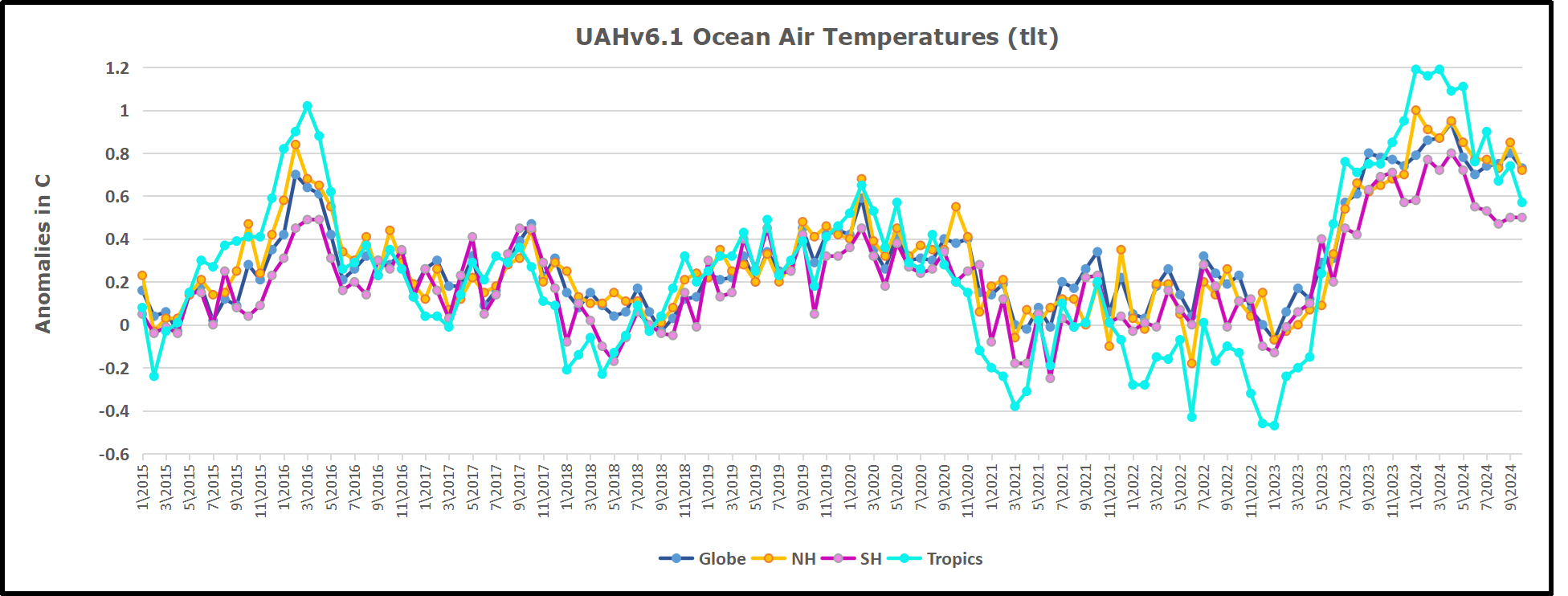
The UAH dataset includes temperature results for air above the oceans, and thus should be most comparable to the SSTs. There is the additional feature that ocean air temps avoid Urban Heat Islands (UHI).  The graph below shows monthly anomalies for ocean air temps since January 2015.

In 2021-22, SH and NH showed spikes up and down while the Tropics cooled dramatically, with some ups and downs, but hitting a new low in January 2023. At that point all regions were more or less in negative territory. 

After sharp cooling everywhere in January 2023, there was a remarkable spiking of Tropical ocean temps from -0.5C up to + 1.2C in January 2024.  The rise was matched by other regions in 2024, such that the Global anomaly peaked at 0.95C in May, Since then the Tropics have cooled down to 0.6C, and the Global anomaly as well as NH dropped down to 0.7C in October.

Land Air Temperatures Tracking in Seesaw Pattern

We sometimes overlook that in climate temperature records, while the oceans are measured directly with SSTs, land temps are measured only indirectly.  The land temperature records at surface stations sample air temps at 2 meters above ground.  UAH gives tlt anomalies for air over land separately from ocean air temps.  The graph updated for October is below.

Here we have fresh evidence of the greater volatility of the Land temperatures, along with extraordinary departures by SH land. The seesaw pattern in Land temps is similar to ocean temps 2021-22, except that SH is the outlier, hitting bottom in January 2023. Then exceptionally SH goes from -0.6C up to 1.4C in September 2023 and 1.8C in August 2024, with a large drop in between. Now in October, NH and the Tropics have pulled the Global Land anomaly down despite a bump in SH land temps.

The Bigger Picture UAH Global Since 1980

The chart shows monthly Global Land and Ocean anomalies starting 01/1980 to present.  The average monthly anomaly is -0.03, for this period of more than four decades.  The graph shows the 1998 El Nino after which the mean resumed, and again after the smaller 2010 event. The 2016 El Nino matched 1998 peak and in addition NH after effects lasted longer, followed by the NH warming 2019-20.   An upward bump in 2021 was reversed with temps having returned close to the mean as of 2/2022.  March and April brought warmer Global temps, later reversed

With the sharp drops in Nov., Dec. and January 2023 temps, there was no increase over 1980. Then in 2023 the buildup to the October/November peak exceeded the sharp April peak of the El Nino 1998 event. It also surpassed the February peak in 2016. In 2024 March and April took the Global anomaly to a new peak of 0.94C.  The cool down started with May dropping to 0.90C, and in June a further decline to 0.80C.  Now in October that temp is down to 0.7C.

The graph reminds of another chart showing the abrupt ejection of humid air from Hunga Tonga eruption.

TLTs include mixing above the oceans and probably some influence from nearby more volatile land temps.  Clearly NH and Global land temps have been dropping in a seesaw pattern, nearly 1C lower than the 2016 peak.  Since the ocean has 1000 times the heat capacity as the atmosphere, that cooling is a significant driving force.  TLT measures started the recent cooling later than SSTs from HadSST4, but are now showing the same pattern. Despite the three El Ninos, their warming had not persisted prior to 2023, and without them it would probably have cooled since 1995.  Of course, the future has not yet been written.

A Kamala Victory Means Green New Deal Lawfare

Expect Kamala Harris’ Justice Department to wage Green New Deal lawfare if she is elected president on Nov. 5.

From Watts Up With That?

By Jason Isaac

Expect Kamala Harris’ Justice Department to wage Green New Deal lawfare if she is elected president on Nov. 5.

As with every last issue pertaining to this election, Harris has not said much about the substance of her climate policy. But a review of her record suggests she’d be amenable to unleashing the Justice Department on energy providers, and her conspicuously quiet allies on the climate left are optimistic she’ll do just that.

Unleashing the Justice Department on American energy companies means hurtling this country deep into the last century. Traditional energy sources are essential for the world historic quality of life most Americans enjoy. Litigation will drive prices up. The lawsuits will also strongarm a transition to electric vehicles, stoves, and water heaters that will remain unpopular with most people because they aren’t affordable and don’t work as well as gas-powered alternatives. Green New Deal lawfare unfolding at the state and local levels all over the country means to force those appliances onto an unwilling public through settlement terms or public spending funded by big money verdicts.

Harris is already aligned with climate lawfare. Harris investigated whether Exxon “repeatedly lied to the public and its shareholders about the risk to its business from climate change” during her tenure as California attorney general, according to the Los Angeles Times. The probe did not result in a lawsuit, though she was supportive of legal claims targeting energy providers as a presidential candidate. 

Harris parroted claims typical of climate lawsuits during her ill-fated 2020 bid. She accused energy providers of concealing inside information about emissions, much as tobacco companies were accused of misleading customers about the health consequences of smoking.

“You should be really prepared to look at a serious fine or be charged with a crime,” Harris said at a 2019 town hall in South Carolina. She made a similar remark in an interview she gave to Mother Jones.

Harris has of course renounced much of her 2020 platform, but climate cultists sense she remains willing to pursue energy providers in court. A coalition of alarmist groups is pushing Harris to direct the Justice Department to investigate the industry, calling such a probe “long overdue.” Democrat partisans like Sheldon Whitehouse and Jamie Raskin are similarly pressuring DOJ to take this step.

One step DOJ could take – and the climate left is already calling for it – is to open a probe under the anti-mafia statute, the Racketeer Influenced and Corrupt Organizations (RICO) Act. That means holding defendants liable not just for emissions, but also for political speech and actions that support a pro-gas energy policy. Democratic lawmakers favorably discussed this avenue in May as a former DOJ official testified to the Senate Budget Committee.

How would anti-energy lawfare cash out for the average American? The cost of settlements or big money verdicts will inevitably reach consumers across numerous points of service. Everything will cost more. You’ll notice this most when paying an energy bill, filling up your tank, or buying a plane ticket. But cheap and abundant energy is essential to all businesses, and there will be hidden penalties everywhere.

Moreover, the climate plaintiffs are already mapping their plans for spending money climate lawfare delivers. These plans include investments in EV-charging infrastructure, mandated electric appliances in new builds, and even repurposing neighborhoods to create 15-minute cities. This is social reengineering by lawsuit, a foisting of lifestyle choices on unwilling participants.

With preelection forecasts favoring a Republican takeover of the Senate, it’s quite likely a president Kamala Harris would not move landmark climate laws through Congress. That means she would have to think creatively about birddogging energy companies, and siccing the Justice Department on them is a likely step. 


Jason Isaac, a former state representative in Texas, is founder and CEO of The American Energy Institute,

This article was originally published by RealClearEnergy and made available via RealClearWire.

Urban Legends of Climate Change: Palm Springs, California

This is the first of what will likely be a series of posts regarding urban heat island (UHI) effects in daily record high temperatures. My previous UHI work has been using the GHCN monthly average station data of “Tavg” (the average of the daily maximum [Tmax] and minimum [Tmin] temperatures). So, I’m moving from Tavg to Tmax (since record high temperatures are of so much interest), and daily rather than monthly values (although I will also sometimes include monthly results to provide context).

From Roy Spencer, PhD

November 5th, 2024 by Roy W. Spencer, Ph. D.

This is the first of what will likely be a series of posts regarding urban heat island (UHI) effects in daily record high temperatures. My previous UHI work has been using the GHCN monthly average station data of “Tavg” (the average of the daily maximum [Tmax] and minimum [Tmin] temperatures). So, I’m moving from Tavg to Tmax (since record high temperatures are of so much interest), and daily rather than monthly values (although I will also sometimes include monthly results to provide context).

This post is mostly a teaser. Toward the end I will describe a new dimension to our UHI work I’m just starting.

The 2024 Poster Child for U.S. Warming: Palm Springs, CA

I was guided by a Google search on U.S. record high temperatures for 2024, and it seems Palm Springs, California was the place to start.

With a name like “Palm Springs” this place sounds like a wonderful spot to lounge under palm trees and enjoy the cool, refreshing spring water that surrounds you. Instead, the location is largely a desert, with the original downtown spring spitting out 26 gallons a minute of hot water. The “palms” do exist… they are “desert palms”, naturally growing in clusters where groundwater from mountain snowmelt seeps up through fissures connected to the San Andreas fault.

Like all U.S. metropolitan areas, the population growth at Palm Springs in the last 100+ years has been rapid. Even in the last 50 years the population has nearly doubled. Natural desert surfaces have been replaced with pavement and rooftops, which reach higher temperatures than the original desert soil, and the “impervious” nature of artificial surfaces (little air content) means the heat is conducted downward, leading to long-term storage of excess heat energy and, on average, higher temperatures. More on “impervious” surfaces later….

The Palm Springs Airport Weather Observation Site

The following Google Earth image shows the current location of the official ASOS (Automated Surface Observing System) site at the Palm Springs Airport, which recorded an all-time record high temperature of 124 deg. F on July 5 of this year.

What is somewhat amusing is that ASOS meteorological instrument siting guidance favors natural surfaces for placement, but since most of these weather stations are at airports (and since they primarily support aviation weather needs, not climate monitoring needs), the “natural” location is usually right next to runways, aircraft, and paved roads.

The next Google Earth image is zoomed out to show the greater Palm Springs area, with the ASOS site in the center (click on the image to zoom, then click to zoom more).

Record July Temperatures and Urbanization

It only makes sense that people want to know the temperature where they live, and most of the U.S. population resides in urban or suburban locations. Yet, the temperatures they experience are, probably without exception, higher than before people moved there and started building roads, buildings, and airports.

But what is misleading for those following the global warming narrative is that record high temperatures reported at these locations almost always mention climate change as a cause, yet they have no way of knowing how much urbanization has contributed to those record high temperatures. (Remember, even without global warming, high temperature records will continue to be broken as urbanization increases).

As mentioned above, on July 5, 2024 Palm Springs broke its all-time high temperature record, reaching 124 deg. F. There are 26 other daily GHCN stations within 40 miles of Palm Springs, all with varying levels of urbanization, but even more importantly, at very different elevations. If we plot the high temperatures reported for July 5 at those stations as a function of station elevation, we see that Palm Springs is an “outlier”, 5 degrees warmer than would be expected based upon its elevation-corrected expected temperature (the dashed regression line):

Now, keep in mind that many (if not most) of those 26 surrounding stations have their own levels of urbanization, making them hotter than they would be in the absence of pavement and roofs. So, that 5 deg. F excess is likely an underestimate of how much urban warming contributed to the Palm Springs record high temperature. Palm Springs was incorporated in 1938, and most population growth there has been since World War II.

If you are curious how the previous plot looks for the average of all July temperatures, here it is:

For the month of July, Palm Springs averaged 3 deg. F warmer than the surrounding stations (after adjusting for elevation effects, and keeping in mind that most of the *other* stations likely have their own levels of urbanization).

Clearly, Palm Springs has had spurious warming influence from the airport and surrounding urbanization which did not exist 100 years ago. But how much?

Impervious Surface Data as a Surrogate for Urbanization

This blog post is a prelude to a new project we’ve started where we will compare daily (as well and monthly) temperatures to a relatively new USGS dataset of yearly impervious surface coverage from 1985 to 2023, based upon Landsat data. I had previously experimented with a “Built Up” dataset based upon Landsat data, but it turns out that was just buildings. The “impervious surface” dataset is what I believe will have the greatest direct physical connection to what causes most UHI warming: roads, parking lots, roofs, etc. I think this will produce more accurate results (despite being only ~40 years in length) than my population density work (which is, we hope, close to being accepted for publication).