How Aligned Climate Cycles Triggered Droughts That Helped Topple Bronze Age Civilizations

The Late Bronze Age Collapse (roughly 1200โ€“1150 BCE) was a dramatic period when many interconnected civilizations in the Eastern Mediterranean and Near Eastโ€”such as the Mycenaean palaces in Greece, the Hittite Empire in Anatolia, Ugarit in Syria, and othersโ€”experienced widespread disruption, destruction, or decline.

The Late Bronze Age Collapse (roughly 1200โ€“1150 BCE) was a dramatic period when many interconnected civilizations in the Eastern Mediterranean and Near Eastโ€”such as the Mycenaean palaces in Greece, the Hittite Empire in Anatolia, Ugarit in Syria, and othersโ€”experienced widespread disruption, destruction, or decline.

Major powers saw palace economies collapse, trade networks break down, cities get destroyed or abandoned, and populations shift. Egypt survived but faced invasions (e.g., by the “Sea Peoples”), while Assyria endured with contractions. It was not a total “dark age” everywhere but marked the end of the Bronze Age palatial system and a transition toward the Iron Age.

Role of Climate: Not the Sole Cause, But a Major Stressor

Climate changeโ€”specifically severe, prolonged droughts (sometimes called a “megadrought”)โ€”is one of the leading factors discussed by researchers. It likely exacerbated other vulnerabilities like economic interdependence, over-reliance on agriculture, political fragility, invasions/migrations (Sea Peoples), possible earthquakes, and social unrest. No single cause explains everything; it was likely a “perfect storm” or systems collapse.

Key evidence for drought:

Pollen records, lake sediments (e.g., Sea of Galilee), speleothems, and tree rings (e.g., juniper in Anatolia) show a shift to drier, more arid conditions around 1250โ€“1100 BCE, one of the driest periods in the Bronze/Iron Age transition.

A particularly acute multi-year drought hit ~1198โ€“1196 BCE (ยฑ a few years), coinciding with the Hittite collapse. Tree-ring data from Anatolia indicate unusually low growth, pointing to failed crops and famine.

This aridity affected rain-fed agriculture in the Levant, Anatolia, and Aegean, leading to crop failures, food shortages, and societal strain. River-based systems (Nile, Tigris-Euphrates) were more resilient.

Droughts likely triggered or amplified migrations, resource conflicts, and the breakdown of trade-dependent economies.

Recent Study (2026): Using EC-Earth to “Unravel” the Climate Mechanisms

A new study from Stockholm University (published in Science Advances, July 2026) used the EC-Earth Earth System Model to simulate Mediterranean climate over the past ~8,000 years. It provides deeper insight into why droughts were so severe then.

Main findings:

  • A long-term gradual drying trend over millennia, driven by slow changes in Earth’s orbital parameters (Milankovitch cycles), set the background.
  • Severe droughts (including those around the Late Bronze Age) occurred when multiple shorter-term natural climate cycles aligned and reinforced each other. These involved variations in the Atlantic Ocean (e.g., circulation patterns) and atmospheric dynamics.
  • This “coincidence” pushed the region past a hydroclimatic threshold, causing more intense aridity than the long-term trend alone would suggest. It reduced moisture from African monsoons and shifted rainfall patterns.

The study links these compounded effects to the pressures on agriculture and societies during the collapse period. It notes the Eastern Mediterranean as a climate “hotspot,” with lessons for modern risks: future droughts may depend on how human-caused warming interacts with natural Atlantic variability.

EC-Earth – A European community Earth System Model

EC-Earth is a state-of-the-art Earth System Model (ESM) developed collaboratively by a European consortium of national meteorological services, research institutes, and universities.

It simulates the Earth’s climate system, including interactions between the atmosphere, oceans, land surface, biosphere, cryosphere, and biogeochemical processes. Researchers use it to study climate variability, climate change, feedbacks, and future projections.

Background and Development

  • The consortium started in 2006.
  • It builds on the ECMWF (European Centre for Medium-Range Weather Forecasts) Integrated Forecasting System (IFS), leveraging expertise from weather prediction for climate modeling (the “seamless prediction” concept).
  • EC-Earth has contributed to major international efforts like CMIP5 and especially CMIP6 (Coupled Model Intercomparison Project Phase 6).

EC-Earth3 (the third generation, used for CMIP6) represents a significant advancement over earlier versions, with improved physics, new Earth system components, better performance, and flexible configurations.

_____________________________________________________________________________________

Holocene ocean-atmosphere coupling and Mediterranean sensitivity to Atlantic circulation: Lessons from the Late Bronze Age collapse

“Holocene ocean-atmosphere coupling and Mediterranean sensitivity to Atlantic circulation: Lessons from the Late Bronze Age collapse” is a 2026 paper by Katherine Power (lead author) and colleagues, published in Science Advances (DOI: 10.1126/sciadv.aed5439).

It uses climate modeling to explore long-term Mediterranean climate dynamics and their relevance to the societal stresses during the Late Bronze Age Collapse (~3200 years ago / ~1200 BCE).

Core Approach and Methods

Researchers employed the EC-Earth Earth System Model (a European community model) to simulate Holocene climate evolution (~last 8,000 years). This allowed reconstruction of ocean-atmosphere interactions, precipitation patterns, and drought variability in the Eastern Mediterranean.

The study focuses on:

  • Long-term orbital forcing (slow changes in Earth’s orbit affecting insolation and seasonality).
  • Internal variability, especially in the Atlantic Ocean (e.g., circulation patterns like aspects of the AMOC or related modes) and atmospheric teleconnections.
  • How these interact across timescales to produce hydroclimatic extremes.

Key Findings

The Eastern Mediterranean experienced a gradual drying trend over the Holocene, driven primarily by orbital changes. This created a background of increasing aridity.

Extreme droughts, including those implicated in the Bronze Age period, arose when multiple natural climate cycles (operating on different timescales) aligned in phase. This reinforcement amplified drying far beyond the long-term trend, pushing the region across critical thresholds for water availability.

Processes involved weakening of moisture transport (e.g., from African monsoons) and shifts in atmospheric circulation linked to Atlantic conditions.

This provides a mechanistic explanation for why droughts around the Late Bronze Age were particularly severe and impactful on agriculture-dependent societies.

The paper frames the Late Bronze Age as a case study (“lessons from”) for understanding Mediterranean climate sensitivity. It highlights the region’s vulnerability to compounded natural variability.

Relevance to the Late Bronze Age Collapse

The modeling supports paleoclimate proxy evidence (tree rings, pollen, sediments) of severe aridity ~1250โ€“1100 BCE. It suggests that aligned climate modes contributed to multi-year to multi-decadal droughts, stressing rain-fed agriculture, causing crop failures and famines, and amplifying societal vulnerabilities (trade disruptions, migrations, political instability).

This aligns with but deepens prior work by offering dynamic explanations rather than just describing the droughts.

Broader Implications

Paleoclimate insight:

Demonstrates the importance of ocean-atmosphere coupling and phase relationships in generating extremes, beyond simple external forcing.

Modern relevance:

The Mediterranean is a climate change hotspot. The study implies that future drought risk depends on the interplay between anthropogenic warming and natural Atlantic variability. Understanding these interactions can improve projections of hydroclimatic extremes.

Data and code are likely available via Zenodo (accompanying dataset mentioned in searches).

This is a strong example of interdisciplinary work bridging high-resolution modeling with archaeology and history.

Journal information: Science Advances

DOI: 10.1126/sciadv.aed5439. www.science.org/doi/10.1126/sciadv.aed5439

Provided: Stockholm University

Authors: Katherine Power and Qiong Zhang

Abstract

Climate variability has profoundly influenced societies in the semiarid Eastern Mediterranean. Proxy records indicate progressive mid-Holocene drying culminating in severe droughts โˆผ1250 BCE, coincident with the Late Bronze Age collapse (1300 to 900 BCE). Using the EC-Earth3-Tr8K transient Holocene simulation, we reconstruct regional hydroclimate evolution and its underlying mechanisms. The model reproduces a gradual orbitally driven aridification, spatially heterogeneous across the region, with persistent drying in the Levant but enhanced effective moisture in parts of the Balkans and Anatolia due to cooling-induced evapotranspiration decline. Superimposed on this long-term trend are extreme drought events, which arise from the alignment of Atlantic internal variability across centennial to millennial timescales, amplifying drying on an already arid background state. These results provide model-based evidence of how evolving amplitude and phase structure of Atlantic internal variability reshaped Eastern Mediterranean hydroclimate through the mid-to-late Holocene. We demonstrate that oceanic variability can manifest as abrupt regional crises when ecological and societal thresholds are crossed.

Temperature Spike Due to Reduced Sulfateย Emissions

After two years of fabricated alarmism about the apparent shift upwards in global temperatures, scientists have now established that the main culprit has been the reduction in sulfate emissions from shipping!

From NOT A LOT OF PEOPLE KNOW THAT

By Paul Homewood

After two years of fabricated alarmism about the apparent shift upwards in global temperatures, scientists have now established that the main culprit has been the reduction in sulfate emissions from shipping!

Abstract

The summer of 2023 saw an anomalous increase in temperatures even when considering the ongoing greenhouse-gas-driven warming trend. Here we demonstrate that regulatory changes to sulfate emissions from international shipping routes, which resulted in a significant reduction in sulfate particulate released during international shipping starting on 1 January 2020, have been a major contributing factor to the monthly surface temperature anomalies during the last year.

We do this by including the appropriate changes to emission databases developed for the Climate Model Intercomparison Project version 6 (CMIP6) in Community Earth System Model (CESM2) simulations. The aerosol termination effect simulated by the updated CESM2 simulations of W mโˆ’2 and 0.08 Kยฑ0.03 K is consistent with observations of both radiative forcing and surface temperature, manifesting a similar delay as the one observed in observational datasets between the implementation of the emission changes and the anomalous increase in warming. Our findings highlight the importance of considering realistic near-future changes in short-lived climate forcers for future climate projections, such as for CMIP7, for an improved understanding and communication of short-term climatic changes.

https://esd.copernicus.org/articles/15/1527/2024

This really should not have come as a surprise to anyone, which strengthens the impression that the climate establishment have deliberately ignored sulfate emissions, in order to focus the publicโ€™s minds on greenhouse gases.

It has long been recognised that sulfate pollution was a factor in the global cooling between the Second World War and the 1970s. As countries began to clean their air, temperatures naturally rose. Even the Met Office admitted this was probably why UK temperatures rose in the 1980s and 90s.

Cornell University have more detail on their researchersโ€™ study:

Mandated reductions in sulfate emissions from international shipping routes in 2020 are partly responsible for the record high temperatures, the researchers found. Reducing the amount of aerosol particles in the atmosphere reduces cloud coverage; thus, cloudsโ€™ ability to reflect solar radiation back to space is diminished. The paperโ€™s findings suggest future policy decisions around abrupt reductions in tropospheric aerosols should take into account their surface temperature impact.

Past research indicated that such change would lead to a minor increase in the global temperature due to a reduction in cloud formation, but Visioni and co-author Ilaria Quaglia, postdoctoral researcher in the Sibley School of Mechanical and Aerospace Engineering (Cornell Engineering), used Earth system model simulations to prove the significance of the sudden drop in sulfate shipping emissions.

These changes in the shipping industry had been discussed for years, Visioni said, with the International Maritime Organization (IMO) making a decision in 2014 to begin enforcing stricter sulfate emissions by 2020. Fuels with lower sulfur are much more expensive, so it took some time for the industry to adjust, he said.

The regulation required ships to use fuel with a sulfur content of no more than 0.5%, down from the previous limit of 3.5%. This reduction led to a more than 80% decrease in total sulfur oxide emissions from shipping.

And while there was some talk of this tradeoff within the shipping industry, he said, there was little attempt to call widespread attention to the potential effect.

The Cornell researchers looked at monthly global temperature anomalies over the period 2020-23, removing the assumed linear contribution from greenhouse gases and seasonality, in order to determine the shipping industryโ€™s impact on temperature anomalies. They found that removing sulfur dioxide from shipping fuel likely increased the planetโ€™s temperature by 0.08 degrees Celsius.

โ€œThe unprecedented heat became a normal warm year once you accounted for that,โ€ Visioni said.

https://news.cornell.edu/stories/2025/01/shipping-emissions-mandate-led-spike-global-temperatures

That last sentence is worth repeating:

โ€œThe unprecedented heat became a normal warm year once you accounted for that,โ€

Japanese Scientist: The IPCCโ€™s Climate Models Are Fundamentally Flawed, Use False Assumptions

There is no theoretical basis for the Net Zero policy based on the man-made climate change narrative of the IPCC. It comes from the lack in knowledge of the atmospheric window of the energy budget of the earthย by modelers.

From NoTrickZone

Byย P Gosselin

By Kyoji Kimoto  

Fig.1 below is an energy budget of the earth having an atmospheric window.

In this case, OLR (Outgoing Longwave Radiation) is expressed as follows.:OLR= Fw (function of Ts, 17%) + Fu (function of Tu, 83%)

Ts โ€“  surface temperature,

Tu โ€“  upper troposphere temperature

Therefore, Tu increases as much as ~1C to restore the decreased OLR as much as 4(W/m2) at the tropopause with a CO2 doubling.

Fig.1. Energy budget of the earth (adapted from Fig.4.1 in Dorland, R.V., de Jager, dr. C.,ย Versteegh, G.J.M., 2006. KNMI Report 50010200, 99-101)

In contrast, climate models were developed by Manabe, Hansen, Cess and Schlesinger using the energy budget of the earth by Fig. 2 having no atmospheric window.

Fig.2. Energy budget of the Earth by Ramanathan (1987)

Therefore 40 climate models participated in CMIP6 have no atmospheric window as shown by Fig. 3. In this case, surface temperature Ts increases as much as ~1C to restore the decreased OLR as much as 4(W/m2) at the tropopause with CO2 doubling.

Fig. 3: Wild (2020) CMIP6 (Coupled Model Intercomparison Project Phase 6)

Fig. 3 All sky was adapted in the following reference: Martin Wild, Climate Dynamics (2020) 55:553-577.

Conclusion

There is no theoretical basis for the Net Zero policy based on the man-made climate change narrative of the IPCC. It comes from the lack in knowledge of the atmospheric window of the energy budget of the earth by modelers.

Theoretically speaking, OLR is treated as one variable function as OLR= function (Ts) in climate models while in reality it is two variable function as OLR= function (Ts, Tu).

A Test of Skill for Climate Models

Do climate models offer a firm basis for attempting to re-engineer the entire global economy?

From Watts Up With That?

Richard Willoughby

The temperature measured across the globe in October 2023 has set a new record high anomaly.  With that as the backdrop, this essay looks at the predictive skill of climate models in forecasting the record.

Anomalies โ€“ A Brilliant Deception

Climate botherers are fixated on temperature anomalies and have convinced sufficient number of voters that 1.5C rise in global average surface temperature (GAST) is a critical threshold for the globe.  October 2023 came perilously close to breaching the threshold so it deserves closer analysis as to what it means and how well various climate models have managed to forecast this outcome.

Temperature of the Lower Troposphere

This analysis begins with the examination of the temperature of the lower troposphere produced by the satellite remote sensing system (RSS) and displayed below in Chart 1.

The data is available atย KNMIย but was last updated in July 2023, which is usually the yearly peak; reaching minus 0.16C in that month.ย  October is typically 2C lower that July.ย  A key feature of Chart 1 is the trend; rising at 2.1C/century.ย  The regression coefficient is only 6.29% due to the significant annual swing in the range 3 to 4 Centigrade degrees.ย  However, if this data is reduced to an anomaly relative to the same month over a 30 year period to iron out the annual variation, the result gets closer to a trend line as shown in Chart 2.

The trend line has almost the same slope; increasing at 2.1C/century as in Chart 1 but now the regression coefficient improves dramatically to 71.4%.  Given the high correlation, it is reasonable to expect this trend to continue for the next 76 years such that the RSS TLT will reach 1.1C in July 2100.  And there are certain to be many more months prior to that year when the 1.5C threshold will be exceeded.  In fact, October 2023 probably exceeded the 1.5C threshold.  The RSS TLT only needed to reach minus 2.85C in October 2023 to exceed the threshold.

Taking A Global Perspective

Reducing the monthly GAST to a single anomalous value is somewhat deceptive.ย  It is as if all surfaces are created equal so it is OK to average them over a whole range of different surface.ย  But this is not based on sound thermodynamic principals.ย  A first step in getting a better appreciation of the significance of record temperatures in 2023 is to examine the warmest month in 2023 with the same month in 1982, the early days of remote satellite sensing to observe how the entire global temperature has responded regionally per Image 1.

The first observation is that the entire globe has not warmed.  Some locations are up to 7.1C cooler than in July 1982 and some are 7.4C warmer.  The warmest regions are in the Northern Hemisphere while the coolest regions are in the Southern Hemisphere.  The area average increase in temperature is 1.3C corresponding to 3.2C/century so slightly above the trend.

Note also that even this satellite determined temperature is not global.  The coldest regions near the poles are excluded from the measurement.

Global Land

It is evident that the thermodynamic response of land surfaces and water surfaces are different.ย  Land responds faster and over a wider temperature range for a given thermal energy input than water.ย  Image 2 indicates the temperature difference from October 1982 to October 2023, the month of highest anomalous GAST, for just land surface, excluding Antarctica, based on the Global Historic Climatology Network (GHCN) measurement.

The area average temperature increase over the land is 2.5C, corresponding to 6.1C per century.  Some land surface has cooled by as much as 4.3C while some warmed by up to 14.1C.  The highest temperature increase is in the high latitudes in the Northern Hemisphere likely to have been permafrost back in 1982.  

Global Ocean

The Reynolds optimally interpolated ocean surface temperature data set is not yet available for the NH summer and fall of 2023 so the ocean surface analysis is stepped back a year by comparing August 2022 to August 1982 as displayed in Image 3.

The increase in area average temperature is 0.5 Centigrade degrees with a range in difference of minus 3.6 to plus 13.1 Centigrade degrees.  The region with the most warming is near the Russian coastline in the Arctic and likely due to earlier annual loss of sea ice in 2022 relative to 1982. 

There are large regions of the oceans in the SH that are now cooler than 1982.  The cool zone along the tropical Pacific was likely warmer in 2023 than 2022 due to El Nino conditions prevailing.  Combining the 0.5C for ocean with the 2.5C for land, gives an area average increase of 1.13C, which is slightly lower than the 1.3C over the same period for the RSS TLT.  It is more than likely that the October 2023 ocean temperature increase is slightly more than 0.5C due to El Nino conditions prevailing in 2023. 

Predictions from Selected Climate Models

The following four images, numbered 4 to 7, compare the predicted results for global temperature based on CMIP6 SSP85 input from various climate prognosticating groups based in regions as follows:

  • ACCESS6 โ€“ Australia
  • INM6 โ€“ Russia
  • MIROC6 โ€“ Japan
  • GISS6 โ€“ USA

The comparison is for October 2023 against the baseline of actual measured values using GHCN for land andย MODISย for ocean surface.ย  MODIS was selected for SST because it is available for October 2023 but has some data gaps observed as greyed pixels in the images.ย  The colour scale for all images is ranged from minus 5 to plus 5 in Centigrade degrees.ย  Regions of red indicate where the model runs hot while blue indicates where the model runs cold.

Compared to measured data, all the models have a tendency to cool the NH and warm the SH.  The scale has a range of ten Centigrade degrees but that was chosen to produce nuanced images.  The variation is much wider for certain locations.  The Greenland Plateau has predicted temperature considerably lower than measured in all models.  The average temperature for each of the four models is:

  • ACCESS6 โ€“ 15.7C
  • INM6 โ€“ 14.7C
  • MIROC6 โ€“ 16.3C
  • GISS6 โ€“ 15.3C

The maximum difference of 1.6C is between the MIROC6 and INM6 models.ย  Image 8 shows how the difference varies across the globe.ย  The difference has a range from minus 9.4 to plus 25.4 Centigrade degrees.ย  The greatest difference is at both poles.

It might be assumed that the MIROC6 model has already reached the dreaded tipping point but the temperature in both polar regions is still well below freezing but just not as cold as the INM6 prediction.

Conclusion

As of October 2023 the difference in average temperature between the models already exceeds the 1.5C threshold and each of the models goes on to predict a future to 2100.  By then the difference in average temperature between the highest and lowest reaches 2.3 Centigrade degrees.  The regional differences between the two models cover a range of 34.8 Centigrade degrees.

The predictive capability of climate models at regional level is far worse than forecasting that any month of next year will be the same as the corresponding month this year.  In fact the measured temperature at any location for any month forty years ago is a better predictor at regional temperature now than any climate model. 

The common difference for all models relative to measured temperature, with the SH running hot and the NH running cold, indicates a systemic error in understanding the natural driver of climate change.  The models are incapable of producing any regional cooling trend so the observed regional cooling trends in the SH invalidate the models.

The notion that regional temperatures across the globe can be averaged to produce the GAST as something meaningful indicates no understanding of thermodynamics.  Debating the difference in GAST from one period to next to a fraction of a degree is mindless nonsense.  The notion the 1.5C increase in GAST will cause a tipping point is in the realm of utter nonsense. 

An Important Question

Do climate models offer a firm basis for attempting to re-engineer the entire global economy?

The Author

Richard Willoughby is a retired electrical engineer having worked in the Australian mining and mineral processing industry for 30 years with roles in large scale operations, corporate R&D and mine development.  A further ten years was spent in the global insurance industry as an engineering risk consultant where he developed an enduring interest in natural catastrophes and changing climate.

Scientists: Nearly 4 Decades Of Climate Model Failure Undermines Confidence In Future Predictions

If the observations of the AMOC are wrong and the multi-model mean of the CMIP6 ensemble
members does represent the twentieth century AMOC, the only problem with the models is
that there is a large range of trends in the CMIP6 ensembles.

From NoTricksZone

By Kenneth Richard on 9. November 2023

IPCC models rooted in assumptions that we humans can and do control the Atlantic Oceanโ€™s circulation with our daily-activity CO2 emissions have been wrong since the mid-1980s. Why should we still believe in them?

The latest IPCC report continues to say it is โ€œvery likelyโ€ the Atlantic Meridional Ocean Circulation (AMOC), a fundamental climate parameter, will weaken (and unleash cooling, catastrophic storms, drought, floods) in the 21st century.

But, as the authors of a new study note, since the mid-1980s the 84 (CMIP5) and 56 (CMIP6) AMOC models have been contradicted by observations in both magnitude and sign. The AMOC has not been declining in response to increases in atmospheric CO2. There is even evidence of trend increases.

โ€œ[W]e find that neither the CMIP5 nor the CMIP6 ensemble mean are successful at representing the observational AMOC data. โ€ฆ We show that both the magnitude of the trend in the AMOC over different time periods and often even the sign of the trend differs between observations and climate model ensemble mean, with the magnitude of the trend difference becoming even greater when looking at the CMIP6 ensemble compared to CMIP5.โ€

So, as the scientists ask, why should we trust future modeled predictions?

โ€œ[I]f these models cannot reproduce past variations, why should we be so confident about their ability to predict the future?โ€

Image Source: McCarthy and Caesar, 2023

Understanding the role of the sun in climate change

Although the sun provides nearly all the energy needed to warm the planet, its contribution to climate change remains widely questioned. Many empirically based studies claim that it has a significant effect on climate, while others (often based on computer global climate simulations) claim that it has a small effect.

From phys.org

By Nicola Scafetta

Figure 1. (A) Anthropogenic (blue) and volcanic (orange) effective radiative forcing functions adopted by the CMIP6 GCMs. (B) Possible solar effective radiative forcing functions. Credit:ย Geoscience Frontiersย (2023). DOI: 10.1016/j.gsf.2023.101650

Although the sun provides nearly all the energy needed to warm the planet, its contribution to climate change remains widely questioned. Many empirically based studies claim that it has a significant effect on climate, while others (often based on computer global climate simulations) claim that it has a small effect.

The Intergovernmental Panel on Climate Change (IPCC) supports the latter view and estimates that almost 100% of the observed warming of the Earth’s surface from 1850โ€“1900 to 2020 was caused by man-made emissions. This is known as theย anthropogenic global warmingย (AGWT) theory.

I addressed this important paradox in a new study published inย Geoscience Frontiers. The conundrum appears to arise from two sets of uncertainties: (i) the historical decades and long-term variations in solar activity are unknown; (ii) the sun may affect Earth’s climate through various physical mechanisms many of which are not fully understood and do not exist in the GCMs.

It is important to notice that the AGWT is based solely on computer simulations of global climate models (GCMs) that use total solar irradiance (TSI) records with very low multidecadal and long-term variability. The same model also assumes that the sun affects the climate system only through radiative forcing such as TSI, although there is evidence that other solar processes may be related to solar magnetic activity (solar wind,ย cosmic rays, interplanetary dust, etc.) also affect the climate.

The total solar irradiance (TSI) records

Decadal and long-term changes in historical solar activity are unknown becauseย total solar irradianceย (TSI) reaching Earth can only be accurately measured by satellites, and these records have only been available since 1978. However, these data remain controversial, as different trends emerge depending on the combination and processing of records provided by different experimental teams.

Solar activity changes over longer periods are modeled using a number of solar activity proxies (e.g. sunspot records, faculae records,ย 14C andย 10Be cosmogenic records, etc.). Proxy models are uncertain for definition, and the result is that theย scientific literatureย has provided a variety of TSI reconstructions that greatly differ from each other in both their secular trends and multidecadal modulation.

I have combined several TSI proxy models, and I have evaluated their effective solar radiative forcing functions to be used for climate studies. Figure 1 compares them along with the volcano and anthropogenic effective forcings. The solar effective forcing functions depicted in Fig. 1B differ in several respects.

The solar forcing function currently used in the CMIP6 GCMs simulations (green) has remained nearly constant for about 200 years and, furthermore, it has decreased progressively from 1970 to 2020. Thus, by using this TSI record, the CMIP6 GCMs could only conclude that the sun could not explain almost any of the warming observed since the pre-industrial period (1850โ€“1900), and particularly that observed from 1980 to 2020.

On the contrary, the other three TSI records (red, yellow, and black) reveal a multidecadal oscillation as well as a clear increasing secular trend that is closely correlated with the changes observed in total surface temperature records.

Figure 2. (A) HadCRUT5 global surface temperature versus the CMIP6 GCM ensemble average. (B) HadCRUT5 global surface temperature versus the proposed empirical modeling of the climate using the alternative solar model. Credit:ย Geoscience Frontiersย (2023). DOI: 10.1016/j.gsf.2023.101650

Modeling the total solar activity (TSA) change effect on the climate

The total sun’s effect on the climate cannot be assessed using only the TSI forcing functions because, for example, alternative solar-related mechanisms have been claimed to directly modulate cloud cover. However, because the physics of such mechanisms is still poorly understood, they cannot be implemented in current GCMs. However, if their impact is shown to be large, current GCMs will be unsuitable to model climate change.

I addressed this issue by assuming that the given TSI records are proxies for totalย solar activityย (TSA) and I adopted an empirical methodology to assess the TSA effect by evaluating its optimal climate fingerprint together with those produced by the anthropogenic and volcanic radiative forcing functions adopted by the CMIP6 GCMs.

The model reproduces the results of the CMIP6 GCMs when their original forcing functions are applied under similar physical conditions. In this case, the equilibrium climate sensitivity (ECS) was 1.4ยฐCโ€“2.8ยฐC, which is compatible with the low-ECS CMIP6 GCM group. This means that about two-thirds of the current GCMs (whose ECS varies between 1.8ยฐC and 5.7ยฐC) are overestimating anthropogenic warming, as other recent studies have confirmed.

However, if the proposed solar records are used as TSA proxies and the climatic sensitivity to them is allowed to differ from the climatic sensitivity to radiative forcings, a much greater solar impact on climate change is found, along with a significantly reduced radiative effect. In this case, the ECS is found to be 0.9ยฐCโ€“1.8ยฐC, with a mean of around 1.3ยฐC. This means that anthropogenic warming is greatly overestimated.

Fig. 2 compares the HadCRUT5 global surface temperature record to (A) the CMIP6 GCM ensemble mean record and (B) the energy balance model using a proposed TSA model that does not use the GCMs’ low-secular-variability TSI record. The GCM simulation depicted in Fig. 2A monotonically warms up (green sketch). On the contrary, the model provided in Fig. 2B indicates an oscillating pattern developing around a warming trend that reproduces the climatic record far more precisely.

This result suggests that about 80% of the solar influence on the climate may not be induced by TSI forcing alone, but rather by other sun-climate processes (e.g., by a solar magnetic modulation of cosmic ray and other particle fluxes, and/or others). These alternative mechanisms must be thoroughly investigated and physically understood before trustworthy GCMs can be created to correctly interpret climate change and produce reliableย climate changeย projections for the future.

This story is part ofย Science X Dialog, where researchers can report findings from their published research articles.ย Visit this pageย for information about ScienceX Dialog and how to participate.More information:ย Nicola Scafetta, Empirical assessment of the role of the Sun in climate change using balanced multi-proxy solar records,ย Geoscience Frontiersย (2023).ย DOI: 10.1016/j.gsf.2023.101650

Prof. Dr. Nicola Scafetta works in the Department of Earth Sciences, Environment and Georesources, University of Naples Federico II, Naples, Italy

A Narrow View Of Rainfall

From Watts Up With That?

Guest Post by Willis Eschenbach

So I came across a news article with the headline:

Philly will have more heat waves, and the Delaware projected to rise more than a foot over the next 25 years

Yeah, right, sez I. The claim is that the flooding will come from increased rainfall in the Philly area. The underlying study is from something named the CRRA:

The Climate Resilience Research Agenda (CRRA) was developed through a collaboration formed in 2019 between the City of Philadelphia, the Delaware Valley Regional Planning Commission (DVRPC), the Academy of Natural Sciences (ANS) of Drexel University, and Drexel University faculty and staff engaged in the Consortium for Climate Risks in the Urban Northeast (CCRUN).

The CRRA Philadelphia folks have put out a document called โ€œA Climate Resilience Research Agenda for the Greater Philadelphia Areaโ€œ, with the subtitle โ€œFindings from 2021 Working Group Discussions And Updated CMIP6 Projections for the Regionโ€. This is the CRRA Philadelphia Findings document, hereinafter โ€œCRRAP Findingsโ€.

Note that these are not findings from scientific studies. Instead, they are CRRAP Findings from โ€œWorking Group Discussionsโ€ and downsampled climate models. Clearly science at its finest โ€ฆ

Inter alia the study says:

Philadelphia is expected to become both hotter and wetter in the future through increased
precipitation, a rising sea level, and increased air temperature. In addition to these changes,
extreme weather in the region is projected to continue to increase in frequency and severity,
leading to increased riverine and stormwater flooding, among other impacts.

I started with the tides. The study shows the following, fromย NOAA.

Figure 1. NOAA sea level rise in Philadelphia

Itโ€™s been rising at 3.04 mm/year, thatโ€™s about an eighth of an inch. And thereโ€™s no sign of acceleration.

Next, here are their projections for future sea levels.

These are relative to the average of the 1995 to 2014 period. For Philadelphia, from the data in Figure 1, that 1995-2014 average is +49 mm. Current sea level there is +95 mm, so itโ€™s gone up by 46 mm since the reference period.

So if itโ€™s going to go up 6 inches by 2035, from today thatโ€™s 6 inches less 46 mm. So it has to go up by 106 mm in the next 11.5 years, which is 9.3 mm per year.

In other words, to get to their lowest estimate of 2035 levels, the Philadelphia sea level rise would have to triple tomorrow and stay that high until 2035. And to get to their highest estimate for 2035, the rate of rise would have to go to 24.7 mm per year tomorrow, and stay there until 2035. Thatโ€™s a sea level rise of almost an inch a year, eight times the current rate, starting tomorrow โ€ฆ yeah, right, thatโ€™s totally legit.

Obviously, these folks just grab numbers and never think to ground-test them against reality.

Next, I got to wondering about the claim of โ€œincreased precipitationโ€. So I went to the marvelous KNMI website and got the six weather stations closest to Philly with over 50 years of rainfall data that extended to the present. These are Philadelphia International Airport, PA; Conshohocken, PA; Neshaminy Falls, PA; Indian Mills 2 W, NJ; Wilmington Porter Rsch, DE; and Lambertville, NJ.

Here are those records:

Figure 3. Monthly rainfall totals, six longterm stations in/near Philadelphia

Hmm โ€ฆ very little trend in there, despite decades of warming. Also, in each case the rain has been decreasing over the last two decades. Finally, we see what is called the โ€œNoah Effectโ€, where one or two of the rainfall totals are much much larger than all the rest. This is a common finding in rainfall data.

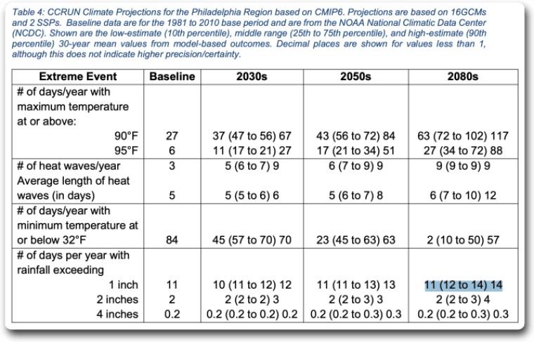
How about their predictions for extreme rainfall? Figure 4 shows those fanciful numbers.

Figure 4. Projections of future extreme events, from the CRRAP Findings.

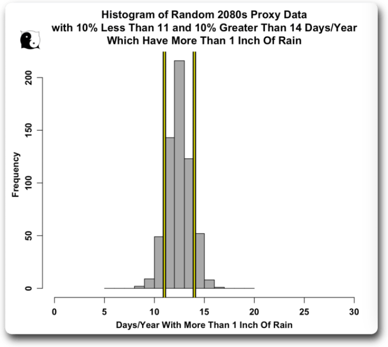
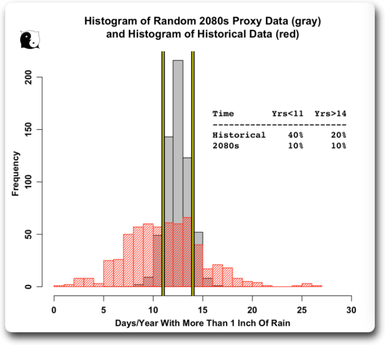
Note the highlighted section. It says that by the 2080s, 10% of the years will have less than 11 days with an inch (25.4 mm) per day of rain, and another 10% of the years will have more than 11 days with an inch per day of rain. Hereโ€™s a histogram of how that might play out.

Figure 5. Random proxy data for the 2080s with 10% under 11 and 10% over 14, as in the CCRAP projections in Figure 4. Yellow/black lines show 11 and 14 days per year.

OK, so thatโ€™s a look at their fantasy for the 2080s โ€ฆ but how does that compare with historical records?

Figure 6 is the same as Figure 5, but it includes a histogram in red of the number of days per year with more than an inch of rain in the six historical records shown above.

Figure 6. As in Figure 5, but includes the historical data in red.

The CMIP6 projections shown in the CRRAP Findings look nothing at all like the historical data. Historically, there are many more years with less than 11 days with an inch of rain. Not only that, but there are more years with more than 14 days with an inch of rain. In fact, in some years, some of the stations recorded over 25 days with more than an inch of rain.

Conclusions? The future projections in the CRRAP Findings document are far from โ€œlife-likeโ€, meaning they bear very little resemblance to actual historical sea level rise and rainfall patterns. If I lived in Philly, Iโ€™d just point and laugh โ€ฆ but hey, I was born yesterday, what do I know?

My best wishes to everyone for a life of love and laughter,

w.

PSโ€”Yeah, Iโ€™m still suspended from Twitter. They claimed it was because I said:

I see that James Comer is going to โ€œtake stepsโ€ against the FBI for concealing evidence of Biden corruption.

Steps? Hereโ€™s my simple 3-step plan.

1) Fire every single person working for the FBI.

2) Burn the FBI building to the ground.

3) Salt the earth.

w.

I stated here on WUWT that I thought it was not because of that tweetโ€”it was for my views on climate. Some people laughed at that idea, claiming it was just my egotism, that the tweeps didnโ€™t care about my climate views, and that my tweet was โ€œinciting violenceโ€.

But a search on โ€œburn down the FBIโ€ (in quotes) on Twitter finds over a hundred tweets, including these two, from folks that arenโ€™t suspended.

So, if youโ€™re on Twitter, maybe you could tweet to @elonmusk to unsuspend @weschenbach โ€ฆ

And Also: When you comment, I implore you to quote the exact words you are discussing, so we can all be clear on your subject.

Epic Fail in Americaโ€™s Heartland: Climate Models Greatly Overestimate Corn Belt Warming

For the last decade Iโ€™ve been providing long-range U.S. Corn Belt forecasts to a company that monitors and forecasts global grain production and market forces. My continuing theme has been, โ€œdonโ€™t believe gloom and doom forecasts for the future of the U.S. Corn Beltโ€.

From ย Roy Spencer, PhD

June 17th, 2023 by Roy W. Spencer, Ph. D.

For the last decade Iโ€™ve been providing long-range U.S. Corn Belt forecasts to a company that monitors and forecasts global grain production and market forces. My continuing theme has been, โ€œdonโ€™t believe gloom and doom forecasts for the future of the U.S. Corn Beltโ€.

The climate models relied upon by the United Nations Intergovernmental Panel on Climate Change (IPCC) are known to overestimate warming compared to observations. Depending upon the region (global? U.S.?), temperature metric (surface? deep ocean? lower atmosphere?) and time period (last 150 years? last 50 years?) the average model over-estimate of warming can be either large or small.

But nowhere is it more dramatic than in the U.S. Corn Belt during the growing season (June, July, August).

The following plot shows the 50-year area-averaged temperature trend during 1973-2022 for the 12-state corn belt as observed with the official NOAA homogenizedย surface temperature productย (blue bar) versus the same metric from 36 CMIP6 climate models (red bars, SSP245 emissions scenario, outputย here).

This kind of sanity check is needed because efforts to change U.S. energy policy are based upon climate model predictions, which are often wildly out of line with observed history. This is why environmentalists emphasize models (which can show dramatic change) over actual observations (which are usually unremarkable).

Is the Antarctic-driven abyssal ocean overturning doomed in 2050?

Probably not, in spite of the recent headlines.

From Climate Etc.

by Frank Bosse

Probably not, in spite of the recent headlines.

A recent article in Nature Abyssal ocean overturning slowdown and warming driven by Antarctic meltwater by England et al. (hereafter E23) caused quite a stir in the media.  The BBC wrote:Antarctic Ocean currents heading for collapse โ€“ report.

E23 built a model to describe the formation and behavior of abyssal water masses around Antarctica.  The Antarctic abyssal waters are important due to its impact on the overturning circulation (AOC) โ€“ the lower cell of the Meridional Overturning Curculation (MOC) โ€“ which overturns heat, freshwater, oxygen, carbon and nutrients in the abyssal ocean.  The AOC directly influences warming and the availability of nutrients to support marine life near the surface of the ocean.

Here is a schematic of the global MOC:

Fig.1.: The global MOC, a reproduction of Fig.1 of Marshall / Speer (2012).  The Antarctic Bottom Water (AABW) is shown on the left side in descending blue arrows.

E23 concludes:

โ€œIn particular, a net slowdown of the abyssal ocean overturning circulation of just over 40% is projected to occur by 205โ€

According to E23, this would also have some impact on the Atlantic Meridional Overturning Circulation (AMOC), which is responsible for the vast majority of the northward heat transport on earth:

โ€œAs the meltwater release from Greenland and Antarctica increases over time, the AABW overturning and AMOC strength both weaken by 2050.โ€ (AMOC by 19% shows Fig. 2).

The cause is the additional meltwater from the Antarctic ice shelves, which has a widespread impact on the Antarctic Bottom Water (AABW):

โ€œFirst, the projected addition of Antarctic meltwater causes an anomalous freshening . . . which produces fresher and less dense AABW, and eventually reduced AABW volume, after the 2030s.โ€

The key figure of E23:

Fig.2: A reproduction of Fig. 3a, b in E23. The Antarctic melting will lead to a reduction under the influence of the anthropogenic forcing (aka โ€œClimate Crisisโ€) of the AABW of 42% (a) in 2050, shown in red. In black: without this forcing.

In Fig. 2 (b) the AMOC shows a robust downward trend over 2004-2020; this is not the case in the observations of โ€œRapidโ€ at 26.5N; ย there is much internal variability, with a dip in 2010 and thereafter a slightly recovery.

Figure:  Observations of the AMOC 2004 to 2020 of โ€œRapidโ€ at 26,5ยฐN:  Source.

Letโ€™s now have a look how the authors calculated the melting up to 2050, which is a crucial input of the described model for the AABW. From the Methods section of E23:

โ€œโ€ฆand the multi-model ensemble mean of CMIP6 models under a high- anthropogenic-emissions scenario, Shared Socioeconomic Pathway 5-8.5 (SSP5-8.5), for the future climate component from 2020 until 2050.โ€

In a twitter thread the lead author stated (and provided a โ€œSharedItโ€ link to read the full paper, thanks for this):

โ€œโ€ฆour projections were run under a โ€˜business as usualโ€™ scenario. Deep and urgent emissions reductions will give us a chance of avoiding an ocean overturning collapse.โ€

Is SSP5-8.5 (or RCP 8.5 in IPCC AR5) โ€œBusiness as usualโ€? Not so, stated this comment, also in โ€œNatureโ€:

โ€œStop using the worst-case scenario for climate warming as the most likely outcomeโ€.

Its projections of future greenhouse gas emissions are generally acknowledged to be unrealistic even on pessimistic assumptions.

Furthermore: is the Multi -Model Ensemble mean (MME) of the CMIP6-models appropriate for this approach? No, the MME mean is skewed high owing to a high climate sensitivity due to some models running much too hot. Gavin Schmidt:

โ€œThe default behavior in the community has to move away from considering the raw model ensemble mean as meaningful.โ€

This leads to an urgent need of a discussion of the choice of SPS5-8.5 and the CMIP6 ensemble mean in E23. Unfortunately the paper doesnโ€™t do this, so I will do it in this blog post.

What effect does the choice of the projected temperatures in the Antarctic for 2020 to 2050 have, which in turn influences the expected melting?

With the help of the KNMI Climate explorer I investigated the expected trends, first for the settings used in E23:

Fig.3: The linear temperature trends in and around Antarctica for SPS5-8.5 and the MMM of the CMIP6โ€™s, as it was estimated in E23.

In comparison, the not-so-skewed CMIP5โ€™s MME mean for the more likely RCP4.5 scenario:

Fig.4: The linear temperature trends for RCP4.5 in and around Antarctica.

Note that the trend slopes in the crucial melting areas of the western Antarctic (including the Ross Sea and the Weddell Sea) are nearly 50% steeper in the Fig. 3 than in Fig. 4. This results in a warming in this area from 2020 to 2050 of 0.6 K (Fig.4) based on RCP 4.5 and the CMIP5 MME mean; in Fig. 3 it results in 1.3 K based on SSP5-8.5 and the CMIP6 MME mean.

However, these are climate model simulation results. Letโ€™s compare the spatially resolved linear trends of grid cells for the area 60ยฐS to 90ยฐS in the time span 1990 to 2021, virtually the same length as the 30 years long time span 2020 to 2050 in E23 for the observations (GISS) and the โ€œnot so hot caseโ€ of Fig.4:

Fig.5: The spatial trend slopes of the gridded data for the CMIP5 models with the scenario RCP 4.5 (left) and observations, GISS (right) for the time span 1990-2021 (โ€œHindcastโ€)

Not only do the simulations warm far too quickly in Antarctica and its environs over the last 30 years,
but the modeled warming is poorly correlated with observed warming in most grid cells (Fig.5)

In wide and crucial areas for the forming of the AABW especially on the coastlines (with the exception of the Ross Sea on the bottom) the observed and modelled trends are quite different โ€“ in the observations the trends are near zero.

The more realistic scenario CMIP5 RCP4.5 shows a twice as fast warming in the Antarctic (60ยฐS-90ยฐS) as the observations, and the CMIP 6-SSP5-8.5 mean scenario shows an almost 3 times faster warming in the โ€œhindcastโ€ period 1990 to 2021 despite the fact that there is relatively little difference in greenhouse gas emissions and changes in other drivers of climate change between the SSP5-8.5 and RCP4.5 scenarios and observations during that period.

In the light uncertainty of the spatial resolved trends in the observations, I use the relation of the trends of the entire Antarctic region, estimating that the warming bias in models will persist to 2050. This would lead to an additional warming of only 0.3K for 2020 to 2050 in the Western Arctic, 23% of the estimation in E23.

Conclusion

Neither the sole warming scenario nor the multi model CMIP6 ensemble mean used by E23 to estimate the melting in Antarctica up to 2050 is appropriate. The resulting MME mean heavily overestimates the likely surface warming and hence the melting, making it โ€œnot meaningfulโ€ (see Gavin Schmidtโ€™s citation) as input for the AABW-model used in E23.

For the crucial regions, the trend slopes 1990 to 2021 in the observations are only about one third of the simulations used by E23. Moreover, projected future greenhouse gas emissions and levels are unrealistically high in SSP5-8.5 scenario used by E23. This suggests that future surface warming in and around Antarctica is likely to be far lower than E23 assumes, which in turn means ice melting and hence the slowing of the abyssal ocean overturning would be much less than E23 projects.

E23 moreover concluded that the ocean freshening due to melting near parts of the western Antarctic (namely Ross Sea and Weddell Sea) will lead to the described reduction of the AABW within 30 years to 2050. I had a look at the observational โ€œArgoโ€ data, provided by the โ€œMarine Atlasโ€. Until December 2021 there is no trend in the salinity data, here shown for the average 0-2000 m depth in the Weddell Sea:

Fig. 6: โ€œArgoโ€ observations of the ocean salinity near the Weddell Sea. In the area of the Ross Sea, there is also no trend (not shown) . The figure was generated with the โ€œMarine Atlasโ€.

The problems with this paper are: reliance on the implausible SSP5-8.5 emissions scenario, use of the CMIP6 multi-model ensemble mean which is running too hot, and failure to critically evaluate the model simulations using recent observations.  Further failures by Natureโ€™s review and editorial process, combined with uncritical and amplified media promotion,  have unnecessarily confused the science and public.

Acknowledgement: I thank Nic Lewis for very helpful comments on earlier draft versions.