Global warming, climate change, all these things are just a dream come true for politicians. I deal with evidence and not with frightening computer models because the seeker after truth does not put his faith in any consensus. The road to the truth is long and hard, but this is the road we must follow. People who describe the unprecedented comfort and ease of modern life as a climate disaster, in my opinion have no idea what a real problem is.
It’s dangerous, *we must* do this that and the other, ambition, fight, requirements etc. When will the tedious climate ranting ever stop? Endless stats come and go, announcing the latest failures of policies supposedly intended to arrange global temperatures to some fraction of a degree. The more they complain, the faster total energy consumption rises, defeating all attempts at control by (as Bill Gates put it) ‘jerking around with renewables’.
It’s dangerous, *we must* do this that and the other, ambition, fight, requirements etc. When will the tedious climate ranting ever stop? Endless stats come and go, announcing the latest failures of policies supposedly intended to arrange global temperatures to some fraction of a degree. The more they complain, the faster total energy consumption rises, defeating all attempts at control by (as Bill Gates put it) ‘jerking around with renewables’. – – – The world is falling dangerously short of the ambition that is needed to secure a safe future climate, according to new analysis by PwC, and as a result we need to fight to prevent every fraction of a degree of warming. [Talkshop comment – fight with what?]
PwC’s latest Net Zero Economy Index shows that a year-on-year decarbonisation rate of 17.2% (up from 15.2% last year) is now required to limit global warming to 1.5°C above pre-industrial levels – seven times greater than what was achieved over the last year (2.5%) and 12 times faster than the global average (1.4%) over the past two decades.
To put this into perspective, since 2000, no G20 country has achieved a decarbonisation rate of more than 11% in a single year – the highest level was achieved by the UK in 2014 (-10.9%).
The Index provides a stark illustration of the growing divergence between the global ambition to tackle climate change and the reality of current progress.
Our analysis shows that all nations need to work harder to reduce emissions to stand any chance of meeting the IPCC’s 2030 deadline to reduce emissions by 43%, with a 78% reduction in carbon intensity now required in under seven years.
Emma Cox, Global Climate Leader, at PwC said:
“The fact the world needs to decarbonise seven times faster is a spur to action, not a counsel of despair. While the overall pace has to pick up rapidly, dramatic change is possible when business and policy makers align. The rapid acceleration of the deployment of wind and solar in several regions shows change can happen. The world is decoupling growth from carbon emissions, now we need that trend to become a surge.”
We notice that when the opposite happens, e.g. heat, storms or more melt happens, then it’s all because of climate warming. But when it goes the other way, then it’s weather!
German research vessel Polarstern of the Alfred Wegener Institute (AWI) is currently underway again in the Arctic. where a decrease in sea ice had been expected there, or, probably more accurately said, hoped for.
But this year the minimum Arctic sea ice extent has turned out differently, as Germany’s widely viewed (climate-alarmist) Tagesschau news had to report:
In view of the extreme summer, the question arose in advance: Will the Arctic also see a new negative record in melting ice this year? This time, the Arctic has been spared. AWI director and expedition leader Antje Boetius tells Tagesschau that an unusual weather phenomenon prevented a record melt of Arctic sea ice this summer. According to Boetius, a sequence of low-pressure systems has led to an entirely different ice movement. The so-called transpolar drift, which describes the drifting of ice along certain routes, took a different course this year, she said. Ice from the Siberian region has been held together and compressed instead of drifting out and melting. For the AWI director, this shows that weather phenomena determine the development of sea ice, and that forecasting is more difficult than ever. The Arctic, with its sea ice and life, has been lucky once again, says the biologist. But things could go the other way. “If we are unlucky, if weather phenomena play unfavorably, we can also be affected by large ice-free parts much sooner than expected,” Boetius adds.”
We notice that when the opposite happens, e.g. heat, storms or more melt happens, then it’s all because of climate warming. But when it goes the other way, then it’s weather!
A very illuminating article was published by a climate scientist, one could say whistleblower, in The Free Press today
The full article is well worth the read. It is a clear indictment of narrative enforcement.
The paper I just published—“Climate warming increases extreme daily wildfire growth risk in California”—focuses exclusively on how climate change has affected extreme wildfire behavior. I knew not to try to quantify key aspects other than climate change in my research because it would dilute the story that prestigious journals like Nature and its rival, Science, want to tell.
This matters because it is critically important for scientists to be published in high-profile journals; in many ways, they are the gatekeepers for career success in academia. And the editors of these journals have made it abundantly clear, both by what they publish and what they reject, that they want climate papers that support certain preapproved narratives—even when those narratives come at the expense of broader knowledge for society.
To put it bluntly, climate science has become less about understanding the complexities of the world and more about serving as a kind of Cassandra, urgently warning the public about the dangers of climate change. However understandable this instinct may be, it distorts a great deal of climate science research, misinforms the public, and most importantly, makes practical solutions more difficult to achieve. https://www.thefp.com/p/i-overhyped-climate-change-to-get-published
Patrick Brown goes in to detail how the scales are tipped to enforce the policy relevant narrative, emphasis mine.
This type of framing, with the influence of climate change unrealistically considered in isolation, is the norm for high-profile research papers. For example, in another recent influential Nature paper, scientists calculated that the two largest climate change impacts on society are deaths related to extreme heat and damage to agriculture. However, the authors never mention that climate change is not the dominant driver for either one of these impacts: heat-related deaths have been declining, and crop yields have been increasing for decades despite climate change. To acknowledge this would imply that the world has succeeded in some areas despite climate change—which, the thinking goes, would undermine the motivation for emissions reductions.
This leads to a second unspoken rule in writing a successful climate paper. The authors should ignore—or at least downplay—practical actions that can counter the impact of climate change. If deaths due to extreme heat are decreasing and crop yields are increasing, then it stands to reason that we can overcome some major negative effects of climate change. Shouldn’t we then study how we have been able to achieve success so that we can facilitate more of it? Of course we should. But studying solutions rather than focusing on problems is simply not going to rouse the public—or the press. Besides, many mainstream climate scientists tend to view the whole prospect of, say, using technology to adapt to climate change as wrongheaded; addressing emissions is the right approach. So the savvy researcher knows to stay away from practical solutions.
Here’s a third trick: be sure to focus on metrics that will generate the most eye-popping numbers. Our paper, for instance, could have focused on a simple, intuitive metric like the number of additional acres that burned or the increase in intensity of wildfires because of climate change. Instead, we followed the common practice of looking at the change in risk of an extreme event—in our case, the increased risk of wildfires burning more than 10,000 acres in a single day.
This is a far less intuitive metric that is more difficult to translate into actionable information. So why is this more complicated and less useful kind of metric so common? Because it generally produces larger factors of increase than other calculations. To wit: you get bigger numbers that justify the importance of your work, its rightful place in Nature or Science, and widespread media coverage. https://www.thefp.com/p/i-overhyped-climate-change-to-get-published
Brown does not pull punches.
To put it another way, I sacrificed contributing the most valuable knowledge for society in order for the research to be compatible with the confirmation bias of the editors and reviewers of the journals I was targeting.
An article in The Los Angeles Times (LA Times) published on September 4, 2023 makes the claim that a study by a Berkeley think tank proves “Climate change has ratcheted up the risk of explosive wildfire growth in California by 25%.” This is false.
An article in The Los Angeles Times (LA Times) published on September 4, 2023 makes the claim that a study by a Berkeley think tank proves “Climate change has ratcheted up the risk of explosive wildfire growth in California by 25%.” This is false. The study ignores other more important factors, and real-world data shows the moisture in the regions of California most affected by wildfires has actually increased, rather than decreased as the study claims.
The LA Times cites a Nature study titled “Climate warming increases extreme daily wildfire growth risk in California.” In the abstract of the paper the authors make an important admission: “Some portion of the change in wildfire behavior is attributable to anthropogenic climate warming, but formally quantifying this contribution is difficult because of numerous confounding factors and because wildfires are below the grid scale of global climate models.”
They also say: “We find that the influence of anthropogenic warming on the risk of extreme daily wildfire growth varies appreciably on a fire-by-fire and day-by-day basis, depending on whether or not climate warming pushes conditions over certain thresholds of aridity, such as 1.5 kPa of vapor-pressure deficit and 10% dead fuel moisture.”
The study fails on these two points because later in the study they cite global climate models using Artificial Intelligence (AI) to tease out relationships that can’t be accounted for in the grid-scale climate models to produce predictions. Models, and especially AI enhanced results are not actual data – they are projections based on the assumptions built into the models and the AI.
The models fail to account for the myriad confounding factors the authors themselves previously acknowledged, such as the increase in arson caused wildfires. In fact, the word “arson” is not mentioned anywhere in the study nor is there any detailed discussion of the actual contributions to increased wildfires of the so-called “confounding factors” in the study.
Ironically, the answer lies in an LA Times article from 2021 which stated: “Electrical equipment accounted for about 12% and lightning 6%. But arson was also a factor, sparking about 9% of fires in 2019, and roughly 8% to 10% of the state’s wildfires in any given year.”
The authors also ignored a 2017 study in the Proceedings of the National Academy of Science (PNAS) which looked at actual data instead of computer models and concluded that in the United States, humans accounted for 84% of wildfires:
Our analysis of two decades of government agency wildfire records highlights the fundamental role of human ignitions. Human-started wildfires accounted for 84% of all wildfires, tripled the length of the fire season, dominated an area seven times greater than that affected by lightning fires, and were responsible for nearly half of all area burned.
A second problematic aspect of the study relates to their use of, “vapor-pressure deficit and 10% dead fuel moisture.” Leaving aside the study’s use of AI enhanced modeling to sift for correlations between small scale moisture changes and wildfire, the researchers also used a novel and little-known approach to link the so-called drought and heat to fossil fuel emissions: Vapor Pressure Deficit (VPD). The VPD is similar to, but not the same as, the more commonly known relative humidity seen in daily weather reports. In layman’s terms, VPD measures how much water is in the air versus the maximum amount of water vapor that can exist in that air. This atmospheric metric is hardly ever used. Climate Realism has refuted the use of VPD to understand drought and wildfire previously.
Most egregious of all, the Nature study itself ignored actual published data about VPD drying. The 2020 paper, Plant responses to rising vapor pressure deficit, examines actual data for the western U.S., specifically in the mountains of California, and shows VPD has decreased, indicating more moisture. These areas show VPD values that indicate more moisture, rather than less, and completely contradict the claims of drying made in the Nature study. This is seen in Figure 1 below, with both the U.S. and an expanded magnified panel showing the western area of the study. The green colors indicate wetter conditions.
Figure 1 – Figure 1A from the paper Plant responses to rising vapor pressure deficit, magnified and annotated by A. Watts to show the Western U.S. and Canada regions cited in the Nature paper. Green areas in California and Western Canada indicate wetter conditions, yet these are areas where the biggest wildfires occurred.
Not only are the authors of the Nature study ignoring the easily available and contradictory VPD evidence in their paper, but they also used global scale climate models to support their assertion that climate change induced VPD deficits are driving wildfires in California, while at the same time admitting the models aren’t suitable for purpose at that scale. Instead, they use AI to tease out fire projections they believe are there but really aren’t.
This is a classic example of the overreliance on models (and now AI) in climate research, instead of actual data. Models are not data, nor do they define reality as actual data does. It is shameful that science and the LA Times present model outputs as such.
Anthony Watts is a senior fellow for environment and climate at The Heartland Institute. Watts has been in the weather business both in front of, and behind the camera as an on-air television meteorologist since 1978, and currently does daily radio forecasts.
He has created weather graphics presentation systems for television, specialized weather instrumentation, as well as co-authored peer-reviewed papers on climate issues. He operates the most viewed website in the world on climate, the award-winning website wattsupwiththat.com.
“The compilation of land- and sea-surface [thermometer] uncertainty yield a 1900-2010 global air-temperature record anomaly of 0.86 ± 1.92°C (2 σ), which renders impossible any conclusion regarding the rate or magnitude of climate warming since 1850 or earlier.” – Dr. Patrick Frank (2023)
“The compilation of land- and sea-surface [thermometer] uncertainty yield a 1900-2010 global air-temperature record anomaly of 0.86 ± 1.92°C (2 σ), which renders impossible any conclusion regarding the rate or magnitude of climate warming since 1850 or earlier.” – Dr. Patrick Frank (2023)
The global surface air temperature record is so contaminated by systematic error (due to solar irradiance, wind speed, albedo reflectance, thermometer physical inadequacies, drift…) that is impossible to distinguish the contaminated from the valid temperatures.
The built-in ± 1.92°C “range of ignorance” in estimating the global temperature changes since 1900 cannot be reduced by averaging, as the errors are clearly not randomly distributed, but instead strongly related to contaminating environmental factors.
A summarizing estimate of the global temperature change since 1900, including the range of ignorance due to error, indicates the 30-year trend was 1.82°C per century from 1971-2000, but 0.0°C per century during 1981-2010, and 1.23°C per century from 1911-1940.
“For SSTs, the available bucket and engine-intake field calibrations show that shipboard SST measurement errors are, likewise, not random. The uncertainties attached to bucket SSTs, 2σ = ±0.4°C and engine-intake SSTs 2σ = ±2°C…”
“Each of the engine-intake calibrations yielded a bias and uncertainty of 0.3 ±1.2°C (1σ), which obviates accuracy.”
“The magnitude of the SST error mean itself remains unknown.”
“The results indicated that a shipboard bucket seawater sample will not accurately convey the physically true sea-surface temperature unless three conditions are simultaneously true: (1) the thermocline is absent; (2) the vessel is heading into the wind; and (3) the mixing layer extends well below the depth of the keel.”
However, the main thing to take away (albeit, of course, this is a report on only a single year’s weather) is that the catastrophic narrative with regard to the UK’s climate seems to be greatly exaggerated.
The prevailing narrative in the mainstream media regarding the UK climate is that it is becoming increasingly chaotic, and we must take urgent steps both to mitigate against climate change (as if we in the UK could do anything meaningful in this regard, while greenhouse gas emissions in much of the world are growing) and to adapt against its effects. That being the case, it is interesting to look at the most recent in a series of reports relating to the UK climate, the report in question being “State of the UK Climate 2021”. This, the eighth in a series of such reports, is probably the most definitive report on this topic, appearing on the Royal Meteorological Society website, and being mostly based, as it says, on:
observations of temperature, precipitation, sunshine and wind speed from the UK land weather station network as managed by the Met Office and a number of key partners and co-operating volunteers.
Given its reliance on data supplied by the Met Office, one might be slightly cautious about this claim:
The observations are carefully managed such that they conform to current best-practice observational standards as defined by the World Meteorological Organization (WMO).
The reasons for caution are set out by Jit here and by Paul Homewood here, here, here and here. Be that as it may, this report is the best we have, so we should look at its findings for 2021 to see how disastrously the UK’s climate is deteriorating in front of our eyes.
The first thing to note is that the most recent 30-year reference period is changed from 1981–2010 to 1991–2020. There is of course a lot of detail, about all aspects of the weather, sea-level and much else, with seasons looked at as much as the year overall. From the executive summary the first piece of information, however, is distinctly underwhelming:
Overall, UK temperature and sunshine for 2021 were near average and rainfall slightly below.
As for land temperature:
2021 was 0.1°C warmer than the 1991–2020 average, and 18th warmest in the UK series from 1884.
But there was quite a bit of seasonal variation, none of which seems to have been predicted, to be predictable, or to be something we can do much to adapt against:
Winter and spring were colder than the 1991–2020 average. However, 2021 included the UK’s ninth warmest summer and equal-third warmest autumn on record in series from 1884.
Despite the most recent decade showing declining days of both ground and air frost, 2021 bucked that trend:
The numbers of air and ground frosts in 2021 were above the 1991–2020 average.
The numbers of air frosts and ground frosts in April 2021 were the highest on record for the UK in series from 1960.
That’s probably bad news, but is the opposite of what we have been told to expect.
On the other hand, this doesn’t look like bad news to be worried about and guarded against:
Heating and cooling degree days in 2021 were near the 1991–2020 average. Growing degree days were seventh highest for the UK in a series from 1960.
As for near-coast sea surface temperature:
2021 was ranked 20th warmest year for UK near-coastal sea-surface temperature (SST) in a series from 1870.
Again, then, a gently warming trend with no great drama in view.
Well surely rainfall must have been significant? After all, this is something the media constantly tell us is becoming more dramatic. Well, not really:
2021 rainfall was 95% of the 1991–2020 average and 102% of the 1961–1990 average.
There were some monthly variations within those statistics, but again nothing that seems to have been predicted or to be readily predictable:
2021 included the UK’s fifth driest April and second wettest May in monthly series from 1836.
Snow is a particularly problematic from of precipitation. What about it?
For a week in early February the UK experienced its most widespread and significant snow event since late February to early March 2018.
In terms of overall snowiness, 2021 was a fairly average year when compared to the last 60 years…
Sunshine, then. Surely there’s some drama here?
The UK 2021 annual sunshine total was 99% of the 1991–2020 average.
But, here it is – the big reveal:
April 2021 was the UK’s equal-sunniest April on record in a series from 1919, shared with April 2020, and also the sunniest calendar month of the year.
Well, it’s definitely getting stormier, isn’t it?
With the notable exception of storm Arwen, the year was less stormy than most other years in recent decades.
There have been fewer occurrences of max gust speeds exceeding 40/50/60 Kt for the last two decades compared to the 1980s and 1990s.
The UK annual mean wind speed for 2021 was second lowest in a series from 1969.
The UK annual mean wind speed from 1969 to 2021 shows a downward trend, consistent with that observed globally.
Oh.
However, this series must be interpreted with some caution.
We aren’t told why it has to be treated with caution, but the need to do so is obvious – it contradicts the prevailing narrative.
What about leaves? They’re a good indicator of a warming climate.
First leaf dates in 2021 were earlier than the baseline (1999–2020) for species that leaf earlier in the season (e.g., Elder normally in March), but delayed by the cold April for later leafing species (e.g., Pedunculate Oak normally in April). This resulted in a mixed spring overall.
Bare tree dates in 2021 were 2–5 days later than normal with Pedunculate Oak pushed back to early December.
Overall, the 2021 leaf-on season was only 1–7 days longer than the 1999–2020 baseline because of the colder spring.
Not a lot to see there, then.
Conclusion
I am being slightly flippant. The detail is very impressive and the report is well worth a read by anyone with an interest in this subject. However, the main thing to take away (albeit, of course, this is a report on only a single year’s weather) is that the catastrophic narrative with regard to the UK’s climate seems to be greatly exaggerated.
Although the sun provides nearly all the energy needed to warm the planet, its contribution to climate change remains widely questioned. Many empirically based studies claim that it has a significant effect on climate, while others (often based on computer global climate simulations) claim that it has a small effect.
Figure 1. (A) Anthropogenic (blue) and volcanic (orange) effective radiative forcing functions adopted by the CMIP6 GCMs. (B) Possible solar effective radiative forcing functions. Credit: Geoscience Frontiers (2023). DOI: 10.1016/j.gsf.2023.101650
Although the sun provides nearly all the energy needed to warm the planet, its contribution to climate change remains widely questioned. Many empirically based studies claim that it has a significant effect on climate, while others (often based on computer global climate simulations) claim that it has a small effect.
The Intergovernmental Panel on Climate Change (IPCC) supports the latter view and estimates that almost 100% of the observed warming of the Earth’s surface from 1850–1900 to 2020 was caused by man-made emissions. This is known as the anthropogenic global warming (AGWT) theory.
I addressed this important paradox in a new study published in Geoscience Frontiers. The conundrum appears to arise from two sets of uncertainties: (i) the historical decades and long-term variations in solar activity are unknown; (ii) the sun may affect Earth’s climate through various physical mechanisms many of which are not fully understood and do not exist in the GCMs.
It is important to notice that the AGWT is based solely on computer simulations of global climate models (GCMs) that use total solar irradiance (TSI) records with very low multidecadal and long-term variability. The same model also assumes that the sun affects the climate system only through radiative forcing such as TSI, although there is evidence that other solar processes may be related to solar magnetic activity (solar wind, cosmic rays, interplanetary dust, etc.) also affect the climate.
The total solar irradiance (TSI) records
Decadal and long-term changes in historical solar activity are unknown because total solar irradiance (TSI) reaching Earth can only be accurately measured by satellites, and these records have only been available since 1978. However, these data remain controversial, as different trends emerge depending on the combination and processing of records provided by different experimental teams.
Solar activity changes over longer periods are modeled using a number of solar activity proxies (e.g. sunspot records, faculae records, 14C and 10Be cosmogenic records, etc.). Proxy models are uncertain for definition, and the result is that the scientific literature has provided a variety of TSI reconstructions that greatly differ from each other in both their secular trends and multidecadal modulation.
I have combined several TSI proxy models, and I have evaluated their effective solar radiative forcing functions to be used for climate studies. Figure 1 compares them along with the volcano and anthropogenic effective forcings. The solar effective forcing functions depicted in Fig. 1B differ in several respects.
The solar forcing function currently used in the CMIP6 GCMs simulations (green) has remained nearly constant for about 200 years and, furthermore, it has decreased progressively from 1970 to 2020. Thus, by using this TSI record, the CMIP6 GCMs could only conclude that the sun could not explain almost any of the warming observed since the pre-industrial period (1850–1900), and particularly that observed from 1980 to 2020.
On the contrary, the other three TSI records (red, yellow, and black) reveal a multidecadal oscillation as well as a clear increasing secular trend that is closely correlated with the changes observed in total surface temperature records.
Figure 2. (A) HadCRUT5 global surface temperature versus the CMIP6 GCM ensemble average. (B) HadCRUT5 global surface temperature versus the proposed empirical modeling of the climate using the alternative solar model. Credit: Geoscience Frontiers (2023). DOI: 10.1016/j.gsf.2023.101650
Modeling the total solar activity (TSA) change effect on the climate
The total sun’s effect on the climate cannot be assessed using only the TSI forcing functions because, for example, alternative solar-related mechanisms have been claimed to directly modulate cloud cover. However, because the physics of such mechanisms is still poorly understood, they cannot be implemented in current GCMs. However, if their impact is shown to be large, current GCMs will be unsuitable to model climate change.
I addressed this issue by assuming that the given TSI records are proxies for total solar activity (TSA) and I adopted an empirical methodology to assess the TSA effect by evaluating its optimal climate fingerprint together with those produced by the anthropogenic and volcanic radiative forcing functions adopted by the CMIP6 GCMs.
The model reproduces the results of the CMIP6 GCMs when their original forcing functions are applied under similar physical conditions. In this case, the equilibrium climate sensitivity (ECS) was 1.4°C–2.8°C, which is compatible with the low-ECS CMIP6 GCM group. This means that about two-thirds of the current GCMs (whose ECS varies between 1.8°C and 5.7°C) are overestimating anthropogenic warming, as other recent studies have confirmed.
However, if the proposed solar records are used as TSA proxies and the climatic sensitivity to them is allowed to differ from the climatic sensitivity to radiative forcings, a much greater solar impact on climate change is found, along with a significantly reduced radiative effect. In this case, the ECS is found to be 0.9°C–1.8°C, with a mean of around 1.3°C. This means that anthropogenic warming is greatly overestimated.
Fig. 2 compares the HadCRUT5 global surface temperature record to (A) the CMIP6 GCM ensemble mean record and (B) the energy balance model using a proposed TSA model that does not use the GCMs’ low-secular-variability TSI record. The GCM simulation depicted in Fig. 2A monotonically warms up (green sketch). On the contrary, the model provided in Fig. 2B indicates an oscillating pattern developing around a warming trend that reproduces the climatic record far more precisely.
This result suggests that about 80% of the solar influence on the climate may not be induced by TSI forcing alone, but rather by other sun-climate processes (e.g., by a solar magnetic modulation of cosmic ray and other particle fluxes, and/or others). These alternative mechanisms must be thoroughly investigated and physically understood before trustworthy GCMs can be created to correctly interpret climate change and produce reliable climate change projections for the future.
This story is part of Science X Dialog, where researchers can report findings from their published research articles. Visit this page for information about ScienceX Dialog and how to participate.More information: Nicola Scafetta, Empirical assessment of the role of the Sun in climate change using balanced multi-proxy solar records, Geoscience Frontiers (2023). DOI: 10.1016/j.gsf.2023.101650
Prof. Dr. Nicola Scafetta works in the Department of Earth Sciences, Environment and Georesources, University of Naples Federico II, Naples, Italy
This report really does undermine the credibility of the claims. The idea that global temperatures could shoot up by 0.22C in the space of three days is physically impossible, El Nino or not. And given that it is all based on computer modelling and used as a propaganda tool makes the whole thing worthless.
The world’s average temperature has reached a new high for the third time in a week, unofficial records show.
Data analysed by a group of US scientists shows the global average temperature on Thursday was 17.23C.
It breaks the 17.01C record set on Monday, surpassed just a day later when the average temperature reached 17.18C.
The temperature readings come from a tool called Climate Reanalyzer. Scientists at the University of Maine use a combination of readings from surface, air balloon and satellite observations as well as computer modelling to assess average global temperatures.
The readings are not an official government record, but they are closely watched as an indicator of how temperatures are fluctuating.
On Thursday the US weather service National Oceanic and Atmospheric Administration (NOAA) said it could not confirm records that come partly from computer simulations, according to Associated Press.
This report really does undermine the credibility of the claims. The idea that global temperatures could shoot up by 0.22C in the space of three days is physically impossible, El Nino or not. And given that it is all based on computer modelling and used as a propaganda tool makes the whole thing worthless.
Meanwhile back in the real world, satellites continue to indicate that global temperature anomalies last month were well below the 1998 and 2016 El Nino peaks:
A 2020 study (Sherwood20) greatly influenced how the IPCC calculated the climate sensitivity. Sherwood20 has been “extremely influential, including in informing the assessment of equilibrium climate sensitivity (ECS) in the 2021 IPCC Sixth Assessment Scientific Report (AR6); it was cited over twenty times in the relevant AR6 chapter“, according to Nic Lewis. A Comment in Nature confirmed this view.1)
A comprehensive explainer of climate sensitivity to CO2
Short summary
According to the Intergovernmental Panel on Climate Change (IPCC), the atmosphere’s climate sensitivity to CO2is likely between 2.5 and 4.0°C. Simply put, this means that (in the very long term) Earth’s temperature will rise between 2.5 and 4.0°C when the amount of CO2 in the atmosphere doubles.
A 2020 study (Sherwood20) greatly influenced how the IPCC calculated the climate sensitivity. Sherwood20 has been “extremely influential, including in informing the assessment of equilibrium climate sensitivity (ECS) in the 2021 IPCC Sixth Assessment Scientific Report (AR6); it was cited over twenty times in the relevant AR6 chapter“, according to Nic Lewis. A Comment in Nature confirmed this view.1)
Nic Lewis took a closer look at this study, and in September 2022, he published his own study (Lewis22) that criticizes Sherwood20. By correcting errors and using more recent data, including from AR6, Lewis22 found that the climate sensitivity may be about 30% lower than what Sherwood20 had found.
If we know what the climate sensitivity is, and if we also know approximately the amount of greenhouse gases that will be emitted going forward, then the amount of future warming that’s caused by greenhouse gases can also be estimated.
In terms of future emissions, a 2022 study (Pielke22) found that something called RCP3.4 is the most plausible emissions scenario. Traditionally, another scenario (RCP8.5), has been used as a business-as-usual scenario, but this is now widely regarded as an extremely unlikely scenario, with unrealistically high emissions.
Assuming that the climate sensitivity from Lewis22 is correct and that RCP3.4 is the most appropriate emissions scenario, then we find that global temperatures will rise by less than 1°C from 2023 to 2100 (not accounting for natural variability).
How much the Earth’s surface air temperature will rise this century depends, among other things, on how sensitive the atmosphere is to greenhouse gases such as CO2, the amount of greenhouse gases that are emitted, and natural variations. It’s hard to predict natural variations, so the focus here will be on climate sensitivity and greenhouse gas emissions (in particular CO2).
Climate sensitivity
Climate sensitivity is the amount of warming that can be expected in the Earth’s surface air temperature if the amount of CO2 in the atmosphere doubles. So if the climate sensitivity is 3°C, and the amount of CO2 in the atmosphere quickly doubles and stays at that level, then the Earth’s surface air temperature will – in the long term – rise by 3°C.2)In the long term, in this case, is more than 1000 years, but most of the temperature increase happens relatively fast.
The exact value for the climate sensitivity isn’t known, and the uncertainty range has traditionally been very large. In 1979, the so-called Charney report found the climate sensitivity to be between 1.5 and 4.5°C. 34 years later, in 2013, the IPCC reached the exact same conclusion – that it’s likely (66% probability) that the climate sensitivity is between 1.5 and 4.5°C. However, the uncertainty in the Charney report may have been underestimated. So even though the official climate sensitivity estimate didn’t change, it wouldn’t be correct to say that no progress was made during those 34 years.
In climate science, there are several different types of climate sensitivity. I won’t go into detail about the various types just yet, but I’ll have something to say about some of them later in the article – when it becomes relevant. The type of climate sensitivity referred to above – in the Charney report and by the IPCC – is called equilibrium climate sensitivity (ECS).
Why so much uncertainty? (Feedback effects)
There’s broad agreement that without so-called feedback effects, the equilibrium climate sensitivity (ECS) would be close to 1.2°C 3), which is quite low and not particularly dangerous. The reason for the great uncertainty comes from how feedback effects affect the temperature.
A feedback effect can be either positive or negative. A positive feedback effect amplifies warming, contributing to a higher climate sensitivity. A negative feedback dampens warming and contributes to a lower climate sensitivity.
The strengths of feedback effects can vary based on the atmosphere’s temperature and composition, and how much of the Earth is covered by ice and vegetation, among other things. Earth’s climate sensitivity is thus not a constant. And for this reason, the equilibrium climate sensitivity, ECS, has been defined as the long-term increase in temperature as a result of a doubling of CO2from pre-industrial levels (which was about 284 parts per million (ppm)).
Atmospheric CO2 concentration currently stands at approximately 420 ppm, which means there’s been a near 50% increase since the second half of the 19th century.4) Since the concentration of CO2 hasn’t yet doubled (and also since the long term is a long way away), the temperature has risen less than than the magnitude of the equilibrium climate sensitivity. To be more precise, the temperature increase has been approximately 1.2°C over the past 150 years.
Water vapor. Increased amounts of greenhouse gases in the atmosphere cause higher temperatures. A higher temperature then allows the atmosphere to hold more water vapor, and since water vapor is a strong greenhouse gas, the increased amount of water vapor in the atmosphere causes the temperature to rise even more.5) The feedback effect from water vapor is therefore said to be positive.
Lapse rate is how the temperature changes with altitude. The higher up you go in the lower atmosphere (troposphere), the colder it gets – on average about 6.5°C colder per kilometer up. So the lapse rate is said to be 6.5°C per kilometer in the lower atmosphere. The feedback from lapse rate is related to the feedback from water vapor, and the two are often considered together. More water vapor causes the temperature to rise more higher up in the atmosphere than closer to the Earth’s surface. This is because the air is generally drier higher up, and so at those altitudes the increased amounts of water vapor has a larger effect on the temperature. The increased temperature at higher altitudes then contributes to more radiation to space, which causes the Earth to cool more. This means that the feedback effect from lapse rate is negative. However, the combined effect of water vapor and lapse rate is positive.
Clouds. Without clouds, the temperature on Earth would be significantly higher than today, but not all clouds have a net cooling effect. Different types of clouds have a different effect on the temperature. On average, high clouds have a warming effect, while low clouds tend to have a cooling effect. When assessing whether total cloud feedback is positive or negative, one must determine whether clouds in a warmer atmosphere on average will have a greater or lesser warming effect than they do now. There is some uncertainty about this, but according to the IPCC, it’s very likely (over 90%) that the feedback effect from clouds is positive, and that therefore changes in cloud cover as a result of increased temperature will amplify the temperature increase.
Surface Albedo Changes. Earth’s surface albedo says how much solar radiation the Earth reflects directly back to space. Currently, it’s around 0.3, which means that the Earth reflects 30% of the incoming solar radiation. The part of the solar radiation that’s reflected does not contribute to warming. The Earth’s albedo can change, for example, when a larger or smaller part of the surface is covered by ice and snow. A higher temperature generally leads to less ice cover, which in turn leads to higher temperatures still, since less radiation is reflected (the albedo decreases). The albedo change resulting from changes in ice cover is a positive feedback effect. (Changes in albedo due to changes in cloud cover are included in the cloud feedback.)
Planck Feedback. A warm object radiates more than a cold object. Or in the case of the Earth: A warm planet radiates more to space than a cold planet. As the Earth warms, it radiates more energy to space, which cools the planet and reduces the rate of warming. The Planck feedback is a strongly negative feedback.6) Actually, the Planck feedback is already included in the calculation of how much the temperature would rise in the absence of (other) feedback effects. In this sense, the Planck feedback is different than the other feedbacks, and it may be best not to think of it as an actual feedback effect, but rather as a fundamental property of physical objects. The Planck feedback is sometimes referred to as Planck response or no-feedback response.
Different ways to calculate climate sensitivity
There are several ways to calculate climate sensitivity. We can base it on the historical record of the past 150 years, where we know approximately how temperature, greenhouse gases, aerosols etc have changed (historical evidence). Or we can estimate the strengths of the various known feedback mechanisms and sum them (process evidence). Or it can be calculated based on how much average temperature has changed since the last ice age glaciation or other warm or cold periods in the Earth’s history (paleo evidence). A fourth possibility is to use climate models – large computer programs that attempt to simulate Earth’s past and future climate under different assumptions.
Sherwood20
In 2020, a large study by 25 authors was published, and it combined the first three of the above-mentioned methods. So they did not calculate climate sensitivity from climate models directly, although the study oftentimes relies on climate models to substantiate some of their values and assumptions.
Sherwood20 concluded that the climate sensitivity is likely (66% probability) between 2.6 and 3.9°C, with 3.1 degrees as the median value. (It’s equally likely that climate sensitivity is higher (50%) or lower (also 50%) than the median.)
The latest IPCC scientific report (AR6) put great emphasis on Sherwood20, and the IPCC, in turn, concluded that climate sensitivity is likely between 2.5 and 4.0°C, a significant narrowing of their previous uncertainty range. (Note, however, that Sherwood20 and the IPCC focused on different types of climate sensitivities, so their respective values aren’t directly comparable.7))
Sherwood20 thoroughly examines all factors that they believe affect climate sensitivity and discusses sources of uncertainty.
Process evidence: Climate sensitivity calculated by adding up feedback effects
The feedback effects that Sherwood20 focused on were primarily the five that I listed earlier. Other feedbacks were estimated as having no net effect. To calculate the climate sensitivity based on feedback effects, the first step is to add up the strengths of each individual feedback effect, and then there’s a simple formula to convert from total feedback strength to climate sensitivity.
The cloud feedback has the largest uncertainty of the various feedback effects. This is true even though the uncertainty has been reduced in recent years.8)
Historical evidence: Climate sensitivity calculated from temperature and other data over the past 150 years
Within some margin of error, we know how the Earth’s surface air temperature has varied over the past 150 years. We also know roughly how the amount of greenhouse gases in the atmosphere has increased – at least since 1958, when the Mauna Loa observatory started measuring atmospheric CO2. But in order to calculate the climate sensitivity to CO2, we also need to know the effect that other drivers of climate change, including aerosols, have had on the temperature and ideally also how the temperature would have changed without human influence. In addition, there’s something called the pattern effect, which, along with aerosols, is what contributes most to the uncertainty in the climate sensitivity when it’s calculated from historical evidence.
Aerosols: Translated from Norwegian Wikipedia, aerosols are “small particles of liquid or solid in the atmosphere, but not clouds or raindrops. These can have a natural origin or be human-made. Aerosols can affect the climate in various complex ways by affecting Earth’s radiation balance and cloud formation. Studies suggest that these have been released since the start of the Industrial Revolution and have had a cooling effect.” The uncertainty in how aerosols affect the temperature is surprisingly large, but they likely have a net cooling effect. The main reason for the large uncertainty is a lack of knowledge about how aerosols interact with clouds.9) Along with greenhouse gases, certain aerosols are released during the combustion of fossil fuels, but with newer technologies, the release of aerosols from combustion is being reduced. If aerosols have a strong cooling effect, it means they’ve counteracted a significant part of the warming from greenhouse gases. If so, the climate sensitivity to CO2 must be relatively high. If the cooling effect from aerosols is smaller, it implies a lower climate sensitivity.
The pattern effect: Different geographical regions have experienced different amounts of warming since the 1800s.10) Following some previous work, Sherwood20 assumes that areas that have experienced little warming will eventually “catch up” with areas that have experienced more warming, and that this will lead to cloud feedback becoming more positive. However, this may not necessarily happen this century.11) There are few climate sensitivity studies prior to Sherwood20 that take the pattern effect into account, and there’s considerable uncertainty about its magnitude. As a result, the uncertainty in the climate sensitivity as calculated from historical evidence is significantly larger in Sherwood20 than in the earlier studies.
Paleo evidence: Climate sensitivity estimated from previous warm and cold periods
Sherwood20 used one past cold period and one warm period to calculate the climate sensitivity based on paleo evidence (past climates). They also looked at one additional warm period (PETM – Paleocene-Eocene Thermal Maximum, 56 million years ago), but didn’t use the results from that period when calculating their main results.
Temperature trends for the past 65 million years. Figure from Burke et al 2018. The original image also contained different future projections, but I’ve removed that part of the image. Note that there are 5 different scales on the time axis.
The cold period that Sherwood20 looked at was the coldest period in the last ice age glaciation (Last Glacial Maximum, LGM), about 20,000 years ago (20 “kyr Before Present” in the graph), when, according to the study, Earth’s temperature was 5±1°C below pre-industrial temperature (so 6±1°C colder than today).
The warm period they looked at was the mid-Pliocene Warm Period (mPWP), about 3 million years ago (3 “Myr Before Present” in the graph), when the temperature was 3±1°C higher than pre-industrial (2±1°C warmer than today).
It may not be obvious that it’s possible to calculate the atmosphere’s climate sensitivity to CO2 based on what the temperature was in previous warm or cold periods. The reason it is possible is that we can also talk about the atmosphere’s climate sensitivity in a more general sense, without specifically taking CO2 into consideration.12) I’ll try to explain.
If the Earth receives more energy than it radiates back to space, the Earth’s temperature will rise. If climate sensitivity is high, the temperature will rise by a relatively large amount. If climate sensitivity is low, the temperature will rise less.
Regardless of what non-temperature factor causes a change in the balance between incoming and outgoing energy – whether it’s due to more greenhouse gases or a stronger sun, or to ice sheets reflecting more sunlight – the result is (approximately) the same. What matters (most) is the size of the change, not what causes it.
So if we know how much warmer or colder Earth was in an earlier time period, and if we also know how much more or less energy the Earth received at that time compared to now, then it should be possible to calculate how sensitive the atmosphere is to a change in incoming energy.
When we know this general climate sensitivity, and when we also know what CO2 does to the atmosphere’s energy balance, then it’s possible to calculate the atmosphere’s climate sensitivity to CO2.
When it comes to what CO2 does to the atmosphere’s energy balance, it’s been found that a doubling of CO2 reduces radiation to space by about 4 watts per square meter (W/m2) over the entire atmosphere.13) Less radiation to space means that more energy stays in the atmosphere, raising temperatures until outgoing radiation again balances incoming radiation.
All of this means that it’s possible (in theory) that the amount of CO2 in the atmosphere was the same today and at an earlier time when temperatures were quite different from today, and even if CO2 levels were the same (and some other factor(s) caused the temperature difference), it would be possible to calculate the atmosphere’s climate sensitivity to CO2 – because we know approximately what a doubling of CO2 does to the atmosphere’s energy balance.
When scientists estimate the climate sensitivity from past warm or cold periods, they’re looking at very long time spans. This means that all the slow feedbacks have had time to take effect, and we can then find the “real” long-term climate sensitivity. Based on what I’ve written earlier, you would probably think this is the equilibrium climate sensitivity, ECS. However, in the definition of ECS, the Earth’s ice cover is kept constant, so ECS is in a way a theoretical – not a real – climate sensitivity. The real long-term climate sensitivity is called Earth system sensitivity, or ESS for short.
The climate sensitivity that Sherwood20 calculated is called effective climate sensitivity (S) and is an approximation of ECS. ECS is likely higher than S, and ESS is likely significantly higher than ECS (so S < ECS < ESS).
Even though ESS is the true very long-term climate sensitivity, S is actually the most relevant climate sensitivity for us, since we’re most interested in what will happen in the relatively near term – the next century or two. Sherwood20 writes:
Crucially, effective sensitivity (or other measures based on behavior within a century or two of applying the forcing) is more relevant to the time scales of greatest interest (i.e., the next century) than is equilibrium sensitivity[.]
As we’ve seen, Sherwood20 combined climate sensitivities from three different lines of evidence (meaning that they combined climate sensitivities that had been calculated in three different/independent ways). For historical and process evidence, Sherwood20 calculated effective climate sensitivity (S). But the type of climate sensitivity that is most easily calculated from paleo evidence is Earth system sensitivity (ESS). So to be able to directly compare, and then combine, the climate sensitivities from all three lines of evidence, they needed to convert from ESS to S.
According to Sherwood20, ESS was around 50% higher than ECS during the mPWP warm period. During the much warmer PETM, Sherwood20 assumed that ESS and ECS were approximately the same since there weren’t any large permanent ice-sheets during that warm period – and hence no significant changes in ice-cover.
For the more recent LGM, however, it was actually possible to calculate ECS directly (instead of ESS), by treating slow feedbacks as forcings rather than feedbacks.14)
Naturally, there’s significant uncertainty involved when calculating climate sensitivity based on previous warm and cold periods (paleo evidence). We don’t know what the Earth’s exact average temperature was, and we also don’t know exactly how much more or less energy the Earth received at that time compared to today (or surrounding time periods). Still, according to Sherwood20, the uncertainty in the climate sensitivity as calculated from paleo evidence isn’t necessarily greater than for the other lines of evidence.
Sherwood20’s conclusion
According to Sherwood20, “there is substantial overlap between the lines of evidence” used to calculate climate sensitivity, and the “maximum likelihood values are all fairly close”, as can be seen in the graph (b) below. (However, the median value for historical evidence has a surprisingly high value of 5.82°C).
This is Figure 20 from Sherwood20 and shows their main results. The figure shows how likely different climate sensitivities (S) are for each of their three lines of evidence – in addition to the combined likelihood (black curve). The higher the curve goes, the greater the likelihood. We see that the most likely value is just under 3°C, but the median value is 3.1°C.
Nic Lewis is a British mathematician and physicist who entered the field of climate science after being inspired by Stephen McIntyre. McIntyre had criticized the perhaps most important study behind the hockey stick graph used in IPCC’s third assessment report from 2001. (See this earlier post I wrote, which talks about the hockey stick controversy, among other things.)
In general, Lewis’ research points to a lower climate sensitivity than IPCC’s estimates.
Here’s a 2019 talk by Nic Lewis on the topic of climate sensitivity. I highly recommend it:
Lewis has published a total of 10 studies related to climate sensitivity, and Sherwood20 referenced studies where Lewis was the main (or only) author 16 times. In September 2022, Lewis published a study, Objectively Combining Climate Sensitivity Evidence, where he discusses and corrects Sherwood20. I will refer to this new study as Lewis22.
In an article that summarizes Lewis22, Lewis argues that Sherwood20’s methodology of combining different lines of evidence to calculate the climate sensitivity is sound:
This is a strong scientific approach, in that it utilizes a broad base of evidence and avoids direct dependence on [Global Climate Model] climate sensitivities. Such an approach should be able to provide more precise and reliable estimation of climate sensitivity than that in previous IPCC assessment reports.
Lewis writes in the article that since 2015, he has published several studies that describe how to combine “multiple lines of evidence regarding climate sensitivity using an Objective Bayesian statistical approach”. Although Sherwood20 was well aware of Nic Lewis’ studies, Sherwood20 had chosen a (simpler) subjective method instead. According to Lewis, the subjective method “may produce uncertainty ranges that poorly match confidence intervals”. Lewis therefore decided to replicate Sherwood20 using the objective method. He also wanted to check Sherwood20’s estimates and data.
The authors of Sherwood20 had, however, made a deliberate choice to use the subjective method. In Schmidt’s article on RealClimate, we can see that Sherwood20 thought the subjective method was more appropriate:
Attempts to avoid subjectivity (so-called ‘objective’ Bayesian approaches) end up with unjustifiable priors (things that no-one would have suggested before the calculation) whose mathematical properties are more important than their realism.
By using the objective method instead of the subjective one, and by also using an appropriate likelihood estimation method,15) the result was actually a slightly higher climate sensitivity. The median climate sensitivity increased from 3.10 to 3.23°C. Lewis comments:
As it happens, neither the use of a Subjective Bayesian method nor the flawed likelihood estimation led to significant bias in Sherwood20’s estimate of [the climate sensitivity] S when all lines of evidence were combined. Nevertheless, for there to be confidence in the results obtained, sound statistical methods that can be expected to produce reliable parameter estimation must be used.
However, after correcting some other errors and using newer data, including from IPCC’s latest scientific report from 2021 (AR6), the most likely value for the effective climate sensitivity fell to 2.25°C. By also using data that Lewis considered as better justified (not newer), the climate sensitivity was revised down by another 0.09°C, to 2.16°C.
The data changes made by Lewis22 are in part explained in the study and in part in an appendix to the study (Supporting Information, S5). In addition to discussing data values that he changed, in the appendix, Lewis also discusses some data values that he conservatively chose not to change – even though he thought Sherwood20’s values weren’t optimal. So a case could actually be made for an even lower effective climate sensitivity than the 2,16°C that Lewis found in his study.
The figure below is taken from Lewis’ summary of Lewis22 and shows Lewis’ results compared to Sherwood20’s:
In (a), (b), and (d), dashed lines represent results from Sherwood20, while solid lines are from Lewis22. In (b), we see that the three lines of evidence for calculating the climate sensitivity coincide nicely for Lewis22, while the variation is slightly larger in Sherwood20. Additionally, the uncertainty is lower (the curves are narrower) in Lewis22, especially for historical evidence (data from the past 150 years). PETM is the warm period that Sherwood20 didn’t include in the calculation of the combined climate sensitivity (PETM = Paleocene-Eocene Thermal Maximum, about 56 million years ago, when temperatures were about 12°C higher than now).
The details: Why Lewis22 found a lower climate sensitivity than Sherwood20
In this section, I’ll try to explain in more detail why Lewis22 found a lower climate sensitivity than Sherwood20. This is the most technical part of this article, and if you’re not interested in the details, you may want to skip ahead to the section on future emissions.
Values with blue text are the same as in IPCC’s latest assessment report (AR6). Values with yellow background in Lewis22 are conservative choices.16) Less conservative choices would have resulted in a lower climate sensitivity. The data changes in Lewis22 are discussed under Review and revision of S20 data-variable assumptions in Lewis22 and in section S5 of Supporting Information.
Historical evidence (data from the past 150 years)
Sherwood20
Lewis22
ΔFCO2
1.731
1.724
ΔFOther well-mixed greenhouse gases
0.969
1.015
ΔFOzone
0.298
0.400
ΔFLand use
-0.106
-0.150
ΔFStratospheric water vapor
0.064
0.041
ΔFBlack carbon on snow and ice
0.020
0.109
ΔFContrails og induced cirrus
0.048
As Sherwood20
ΔFSolar
0.017
0.019
ΔFVolcanic
-0.113
0.044
ΔFAerosols
-1.104
-0.860
ΔF (sum, difference in forcing, W/m2)
1.824
2.390
ΔN (W/m2)
0.600 ± 0.183
As Sherwood20
ΔT (or ΔTGMAT, °C)
1.03 + 0.085
0.94 ± 0.095
λhist (W/m2/°C)
-1.188
-1.915
𝛾 (scaling factor)
Omitted (1.00)
0.86 ± 0.09
ΔF2xCO2 (W/m2)
4,00 ± 0,30
3.93 ± 0.30
Δλ (pattern effect, W/m2/°C)
0.500 ± 0.305
0.350 ± 0.305
Climate sensitivity, S (°C)
5.82
2.16
ΔF, ΔN, and ΔTGMAT refer to differences between 1861-1880 and 2006-2018. ΔF is the difference in climate forcing (climate forcing (or radiative forcing) is something that forces the Earth’s energy balance to change, e.g. a stronger/weaker sun or more/less greenhouse gases in the atmosphere). ΔN is the change in radiative imbalance at the top of the atmosphere, measured in W/m2. A positive ΔN means that the radiative imbalance is greater now than at the end of the 19th century, and that the Earth is receiving more net energy now than then.
The exact ΔF values that Lewis22 uses can’t be found in IPCC AR6. The reason for this is that Sherwood20 and Lewis22 look at the period from 1861-1880 to 2006-2018, while the IPCC has been more interested in the period 1750 to 2019. Fortunately, though, IPCC has also included forcing values for 1850 and also for several years after 2000, so Lewis has been able to calculate ΔF values with good accuracy (derived from official IPCC values, see table AIII.3 here).
GMAT (Global Mean near-surface Air Temperature) is average air temperature above ground. GMST (Global Mean Surface Temperature) is the same but uses sea surface temperature instead of air temperature over the ocean. Sherwood20 converted ΔTGMST (0.94°C) to ΔTGMAT (1.03°C) based on results from climate models, which suggest that GMAT is higher than GMST. Lewis, however, points out that a higher GMAT than GMST hasn’t been observed in the real world, and that, according to the IPCC AR6, the best estimate median difference between GMST and GMAT is 0. Lewis22 therefore uses a value for ΔTGMAT that’s equal to ΔTGMST. (See Supporting Information, 5.2.1.)
When estimating effective climate sensitivity (S) from climate feedback (λ), a scaling factor 𝛾 (gamma) is needed (for historical and process evidence). This is because Sherwood20 used linear regression to estimate S based on the ratio of ΔN to ΔT, a relationship that isn’t strictly linear. The reason it’s not linear is that, according to most climate models, climate feedback (λ) weakens during the first decade following a sudden increase in CO2. (That λ weakens means it gets closer to 0 (less negative), which means that climate sensitivity, S, increases.)
Sherwood20] recognize this issue, conceding a similar overestimation of S, but neglect it, asserting incorrectly that it only affects feedback estimates from [Global Climate Models]. This misconception results in [Sherwood20]’s estimates of S from Process and Historical evidence being biased high.
Lewis22 used numbers from the two most recent generations of climate models (CMIP5 and CMIP6) to determine that 𝛾 = 0.86.
The reason for the relatively large change in aerosol forcing (ΔFAerosols) is quite elaborate and advanced, so for that I’ll have to refer you to the Supporting Information (5.2.3, starting from the third paragraph).
The change Lewis22 made for the pattern effect (Δλ) is in large part done because most datasets for sea surface temperature point to the so-called unforced component of the pattern effect (having to do with natural variation, see footnote 8) being very small. See Supporting Information, 5.2.4.
Process evidence (Adding up feedback effects):
Sherwood20
Lewis22
λWater vapor + lapse rate
1.15 ± 0.15
As Sherwood20
λCloud
0.45 ± 0.33
0.27 ± 0.33
λAlbedo
0.30 ± 0.15
As Sherwood20
λPlanck
-3.20 ± 0.10
-3.25 ± 0.10
λOther
0.00 ± 0.18
As Sherwood20
λ (Sum, feedback effects, W/m2/°C)
-1.30 ± 0.44
-1.53 ± 0.44
𝛾 (Scaling factor)
Omitted (1.00)
0.86 ± 0.09
ΔF2xCO2 (W/m2)
4.00 ± 0.30
3.93 ± 0.30
Climate sensitivity, S (°C)
3.08
2.21
Lewis adjusted the cloud feedback (λCloud) down based on data from Myers et al 2021 (a more recent study than Sherwood20), which found a lower value for low-cloud feedback over the ocean (0-60° from the equator). According to Myers et al 2021, the low-cloud feedback strength is 0.19 W/m2/°C, while Sherwood20 had used 0.37. The difference of 0.18 is how much the total cloud feedback strength was adjusted down in Lewis22. See Supporting Information (5.1.3) for more details.
According to physical expectation (calculated from a formula) and also the latest climate models (CMIP6), the Planck feedback (λPlanck) is -3.3 W/m2/°C. Sherwood20 acknowledged that the physical expectation for the Planck feedback is -3.3, but they put more weight on the previous generation of climate models (CMIP5) and used -3.2 as the value for the Planck feedback. Lewis22 adjusted the Planck feedback halfway from Sherwood20’s estimate towards the value from physical expectation and CMIP6. See Supporting Information (5.1.2).
As a curiosity, the strength of the albedo feedback here has the same numerical value as the Earth’s albedo, namely 0.30. That’s merely a coincidence.
Paleo evidence (past cold and warm periods)
The coldest period during the last ice age glaciation (Last Glacial Maximum, LGM)
Sherwood20
Lewis22
ζ (how much higher ECS is than S)
0.06 ± 0.20
0.135 ± 0.10
ΔFCO2
-0.57 x ΔF2xCO2 = -2.28
-0.57 x ΔF2xCO2 = -2.24
ΔFCH4
-0.57
As Sherwood20
ΔFN2O
-0.28
As Sherwood20
ΔFLand ice and sea level
-3.20
-3.72
ΔFVegetation
-1.10
As Sherwood20
ΔFDust (aerosol)
-1.00
As Sherwood20
ΔF (difference i forcing, W/m2)
-8.43 ± 2.00
-8.91 ± 2,00
ΔT (difference in temperature, °C)
-5.0 ± 1.00
-4.5 ± 1,00
α (state dependence)
0.10 ± 0.10
As Sherwood20
λ (W/m2/°C)
-1.522
-1.992
ΔF2xCO2 (W/m2)
4.00 ± 0.30
3.93 ± 0.30
Climate sensitivity, S (°C)
2.63
Sherwood20 calculated ζ (zeta; how much higher equilibrium climate sensitivity, ECS, is than the effective climate sensitivity, S) by looking at abrupt 4xCO2 simulations – computer simulations where the atmosphere’s CO2 level is instantaneously quadrupled. Sherwood20 then divided the resulting climate forcing (ΔF4xCO2) by 2 to find the climate forcing for a doubling of CO2 (ΔF2xCO2). Lewis22 notes that the scaling factor of 2 “while popular, is difficult to justify when the actual [scaling factor] has been estimated with reasonable precision to be 2.10”. However, Lewis did not use this method to calculate ζ – instead, he extracted the ζ value (0.135) directly from the results of climate models (or, to be more precise, from long-term simulations by climate models of warming after CO2 concentration was doubled or quadrupled, finding the same value in both cases). More details can be found under Climate Sensitivity Measures in Lewis22.
ΔF is the difference in climate forcing between the coldest period of the last ice age glaciation and pre-industrial times. ΔT is the temperature difference between these periods.
Sherwood20’s ΔT estimate was 5.0°C. However, the mean ΔT value for the studies that Sherwood20 based their estimate on was only 4.2°C (after, where necessary, adjusting values given in the studies to fairly reflect an observational (proxy-based) estimate of the temperature (GMAT) change). Lewis22 therefore adjusted Sherwood20’s ΔT estimate towards that value, from 5.0 to 4.5°C. See Supporting Information, 5.3.2.
The reason for Lewis22’s revision of ΔFLand ice and sea level was that Sherwood20 had omitted albedo changes resulting from lower sea levels. (The sea level was approximately 125 meters lower during the LGM than now, so Earth’s land surface was larger during the LGM than now. Land reflects more solar radiation than water, so the Earth’s albedo might have been higher during the LGM than what Sherwood20 assumed.) See Supporting Information, 5.3.2.
α (alpha) says something about how climate sensitivity varies based on the state of Earth’s climate system. What we’re most interested in is the climate sensitivity for the current and near-future states of the climate system. Since climate sensitivity may be different for warm periods than cold periods (possibly higher in warm periods), we need to convert the climate sensitivity for any past warm or cold period to the current climate sensitivity. The α parameter is included in an attempt to translate the climate sensitivity for the LGM cold period into the current climate sensitivity.
In contrast to Sherwood20’s assumption about the state dependence, Lewis22 writes that a 2021 study by Zhu and Poulsen “found that ocean feedback caused 25% higher LGM-estimated ECS.” This would bring the LGM climate sensitivity closer to the current climate sensitivity. For this reason (and one other) Lewis thought Sherwood20’s estimate for α was questionable. Still, he retained it. See Supporting Information, 5.3.2 (last paragraph).
Mid-Pliocene Warm Period (mPWP)
Sherwood20
Lewis22
CO2 (ppm)
375 ± 25
As Sherwood20
ΔF2xCO2 (W/m2)
4.00 ± 0.30
3.93 ± 0.30
ΔFCO2 (difference i forcing from CO2, W/m2)
1.604
1.576
ζ (how much higher ECS is than S)
0.06 ± 0.20
0.135 ± 0.10
fCH4
0.40 ± 0.10
As Sherwood20
fESS
0.50 ± 0.25
0.67 ± 0.40
ΔT (°C)
3.00 ± 1.00
2.48 ± 1.25
λ (W/m2/°C)
-1.190
-1.686
Climate sensitivity, S (°C)
3.36
2.33
ΔT is the difference in temperature between the mid-Pliocene Warm Period (mPWP) and pre-industrial times. A positive value for the temperature difference means that mPWP was warmer. ΔFCO2 is the difference in climate forcing (from CO2) between mPWP and pre-industrial. fCH4 is the estimated forcing change from methane (and actually also N2O/nitrous oxide) relative to the forcing change from CO2 (so if the forcing change from CO2 is 1.6, then the forcing change from CH4 (and N20) is 0.64). fESS is how much higher the climate sensitivity ESS is compared to the climate sensitivity ECS. The number 284 in the formula represents the pre-industrial CO2 level (measured in parts-per-million).
Lewis22 used a newer value for fESS than Sherwood20. Sherwood20 obtained the value of 0.50 (or 50%) from The Pliocene Model Intercomparison Project (which focuses on the Pliocene era) version 1 (PlioMIP1). The value of 0.67 (or 67%) used by Lewis22 was taken from PlioMIP2, a newer version of the PlioMIP project. See Supporting Information, 5.3.3.
The change Lewis22 made to ΔT was also based on PlioMIP2. Tropical temperatures during the mPWP were about 1.5°C higher than pre-industrial tropical temperatures. To determine the change in global temperature, Sherwood20 multiplied the change in tropical temperatures by 2 on the grounds that average global temperature has changed about twice as much as tropical temperature over the last 500,000 years. However, conditions on Earth were different during the mPWP three million years ago, with much less extensive ice sheets than at present. The PlioMIP2 project has used climate models to estimate that changes in global temperature may have been about 1.65 times higher than changes in tropical temperature during the Pliocene. Lewis22 used this value and consequently multiplied the tropical temperature change (1.5°C) by 1.65 instead of by 2. This changes ΔT from 3.00°C down to 2.48°C. See Supporting Information, 5.3.3.
Paleocene–Eocene Thermal Maximum (PETM):
Using β = 0, we can simplify to:
Sherwood20
Lewis22
ζ
0.06 ± 0.20
0.135 ± 0.10
ΔT (°C)
5.00 ± 2.00
As Sherwood20
fCH4
0.40 ± 0.20
As Sherwood20
CO2 (ppm)
2400 ± 700
As Sherwood20
β
0.0 ± 0.5
As Sherwood20
fCO2nonLog
Omitted (1.00)
1.117
Climate sensitivity, S (°C)
2.38
1.99
ΔT refers to the difference in temperature between the Paleocene-Eocene Thermal Maximum (PETM) and the time just before and after the PETM. During the PETM, temperatures were about 13°C higher than pre-industrial temperatures. Just before and after the PETM, temperatures were about 5°C lower than this (8°C higher than pre-industrial). The number 900 in the formula represents the approximate CO2 level before and after the PETM. fCH4 is again the estimated difference in climate forcing from methane (and nitrous oxide) relative to the forcing change from CO2.
Sherwood20 assumes that the relationship between CO2 concentration and CO2 forcing is logarithmic. Lewis refers to Meinshausen et al. 2020, the results of which were adopted by the IPCC in AR6, which found that at high CO2 concentrations (such as during the PETM), the climate forcing is higher than if the relationship had been purely logarithmic. By using a formula from Meinshausen, Lewis found that the CO2 forcing during the PETM would have been some 11.7% higher than Sherwood20’s assumption of a purely logarithmic relationship. Therefore, Lewis22 used a value of 1.117 for fCO2nonLog. See Supporting Information, 5.3.4.
One would think that a higher CO2 forcing at high temperatures would imply a higher climate sensitivity during warm periods, but that’s not necessarily true, since feedback strengths may be different in warm and cold periods. However, if feedback strengths are the same in warm and cold periods, then a higher CO2 forcing implies a higher climate sensitivity.
Sherwood20 then assumes that the climate sensitivity ESS during the PETM is roughly the same as today’s equilibrium climate sensitivity, ECS. Uncertainty is accounted for with the parameter β, whose mean value is set to zero. Lewis agrees that “[a]ssuming zero slow feedbacks in the PETM (so ESS equals ECS) may be reasonable, given the lack of evidence and the absence of major ice sheets.” However, some studies (that rely on climate models) suggest that climate sensitivity during the PETM may have been higher than it is today. For this reason, Lewis thinks a positive mean value for β would be better. He nonetheless retained Sherwood20’s estimate of zero. See Supporting Information, 5.3.4.
This concludes the most technical part of this article. Next up: greenhouse gas emissions.
To determine how much the temperature will rise in the future (disregarding natural variability), it’s not enough to know what the climate sensitivity is – we also need to know approximately how much greenhouse gases will be emitted, so:
What will the emissions be?
The media and many scientists have long used something called RCP8.5 as a business-as-usual scenario for the effect of human activity (including emissions of greenhouse gases), and many still do. RCP stands for Representative Concentration Pathway, and the number (8.5 in this case) is how much greater the net energy input to the atmosphere is in the year 2100 compared to pre-industrial levels, measured in W/m2.
But RCP8.5 was never meant to be a business-as-usual scenario. In a 2019 CarbonBrief article about RCP8.5, Zeke Hausfather, another co-author of Sherwood20, writes:
The creators of RCP8.5 had not intended it to represent the most likely “business as usual” outcome, emphasising that “no likelihood or preference is attached” to any of the specific scenarios. Its subsequent use as such represents something of a breakdown in communication between energy systems modellers and the climate modelling community.
Sherwood20 also mentions that RCP8.5 should not be seen as a business-as-usual scenario, but rather as a worst-case scenario:
Note that while RCP8.5 has sometimes been presented as a “business as usual” scenario, it is better viewed as a worst case (e.g., Hausfather & Peters, 2020).
RCPs are often referred to as scenarios, which I also did earlier. But it may be better to think of an RCP as a collection of scenarios that all result in roughly the same net change in incoming energy in the year 2100. Thousands of different scenarios have been developed, and these can be used as inputs to climate models when they simulate future climates.
Plausible emissions scenarios
Roger Pielke Jr, Matthew Burgess, and Justin Ritchie published a study in early 2022 titled Plausible 2005–2050 emissions scenarios project between 2 °C and 3 °C of warming by 2100. In Pielke22, the different scenarios used in IPCC’s 2013 assessment report were categorized based on how well they were able to predict actual emissions from 2005 to 2020, in addition to how well their future emissions matched the International Energy Agency’s projections until 2050. Assuming that the scenarios that best matched actual and projected emissions will also be the ones that will be best at predicting emissions in the second half of the century, they found that RCP3.4 is the most likely (or plausible) RCP.
These scenarios (RCP3.4) are largely compatible with a temperature increase of between 2 and 3°C from pre-industrial times to 2100, with 2.2°C as the median value. Earth’s average temperature has increased by about 1.2°C since pre-industrial, so the median of 2.2°C corresponds to a temperature increase from today to 2100 of about 1.0°C.
After Pielke22 was published, Pielke Jr also looked at the scenarios used in IPCC’s latest assessment report (from 2021). He spoke about this in a talk in November 2022 (54:03-1:06:16), and, according to Pielke Jr, the median value for these newer scenarios is 2.6°C (rather than 2.2°C). This corresponds to a temperature rise of 1.4°C from today until 2100. In the following, I will use this more recent value.
In the talk, Pielke Jr says that RCP4.5 should now be considered a high-emissions scenario, while RCP8.5 and RCP6.0 are unlikely (58:12):
The high emissions scenarios are clearly implausible […]. What’s a high emissions scenario? Anything over 6 W/m2 […].
RCP 4.5 and the SSP2-4.5 are plausible high emissions scenarios. I know in the literature they’re often used to represent mitigation success. Today I think we can say based on this method that they’re in fact high-end scenarios. A business as usual – or consistent with current policy – scenario is a 3.4 W/m2 scenario. I will say that scenario is almost never studied by anyone.
Pielke22 doesn’t mention climate sensitivity explicitly, but the median equilibrium climate sensitivity (ECS) used in the latest generation of climate models is 3.74°C. ECS is likely higher than the effective climate sensitivity (S), which is the type of climate sensitivity that Sherwood20 and Lewis22 calculated. According to Sherwood, ECS is 6% higher than ECS. According to Lewis22, ECS is 13.5% higher. Using Lewis22’s value of 13.5%, an ECS of 3.74°C corresponds to an effective climate sensitivity (S) of 3.30°C.
If the climate sensitivity S is closer to 2.16°C, as Lewis22 found, then the temperature increase from today to 2100 will be approximately 35% lower than what Pielke Jr found. This means that the temperature increase from today will be 0.9°C instead of 1.4°C (0.9°C higher than today will be 2.1°C above pre-industrial).
An assumption in the RCP3.4 scenarios is widespread use of CO2 removal from the atmosphere in the second half of the century. Pielke22 did not assess whether that’s feasible:
Importantly, in the scenarios our analysis identifies as plausible, future decarbonization rates accelerate relative to the present, and many include substantial deployment of carbon removal technologies in the latter half of the century, the feasibility of which our analysis does not assess.
Given the recent rapid pace of technological development, I believe it to be highly likely that potent CO2 removal technologies will be developed this century. However, other methods may be more economically effective in limiting an unwanted temperature rise, e.g. manipulating the cloud cover, as Bjørn Lomborg suggests in an interview on Econlib (skip forward to 8:35 and listen for 2 minutes or read in footnote 17)).
In October 2022, The New York Times published an extensive article titled Beyond Catastrophe – A New Climate Reality Is Coming Into View. According to the author, David Wallace-Wells, recent evidence shows that the Earth is on track for a 2-3°C warming from the 1800s until 2100 instead of the previously feared 4-5°C. 2-3°C is the same as Pielke22 found.
According to The New York Times article, Hausfather contends that about half of the reduction in expected temperature rise is due to an unrealistic scenario being used previously (RCP8.5). The other half comes from “technology, markets and public policy”, including faster-than-expected development of renewable energy.
How much will temperatures rise by 2100?
Figure 1 (b) in Sherwood20 (graph (b) below) shows how much the temperature is likely to rise between 1986-2005 and 2079-2099, depending on effective climate sensitivity (S) and RCP scenario. This period is about 16 years longer than the 77 years from today until 2100, so the temperature rise for the remainder of the century will be less than the graph suggests – about 18% lower if we assume a linear temperature rise.
We can see in the graph that if RCP4.5 is the correct emissions scenario and the effective climate sensitivity is 3.1°C, then the temperature will rise by about 1.8°C between 1986-2005 and 2079-2099. To estimate the temperature rise from today until 2100, we subtract 18% from 1.8°C, resulting in an estimated increase of about 1.5°C.
Using instead Lewis22’s effective climate sensitivity of 2.16°C with the RCP4.5 scenario, we can see from the graph that the temperature increase will be approximately 1.25°C. This corresponds to a temperature rise of 1.0°C from today until 2100.
RCP3.4 is not included in the graph, but we can assume that the temperature increase for RCP3.4 will be a few tenths of a degree lower than for RCP4.5, so perhaps 0.7-0.8°C, which also agrees quite well with what Pielke Jr found (0.9°C) after we adjusted for the climate sensitivity from Lewis22.
0.8°C corresponds to a temperature rise of 2.0°C since the second half of the 19th century and is identical to the Paris agreement’s two degree target. 2.0°C is also within the New York Times interval of 2-3°C, where – as for the two degree target – pre-industrial is the starting point.
Although Lewis22’s estimate of climate sensitivity may be the best estimate as of today, it’s not the final answer. Much of the adjustment made to Sherwood20’s estimate was based on more recent data, and as newer data becomes available in the future, the effective climate sensitivity estimate of 2.16°C is going to be revised up or down.
And Nic Lewis points out that:
This large reduction relative to Sherwood et al. shows how sensitive climate sensitivity estimates are to input assumptions.
But he also criticizes the IPCC for significantly raising the lower end of the climate sensitivity likely range (from the previous to the latest assessment report, the lower end of the likely range was raised from 1.5 to 2.5°C):
This sensitivity to the assumptions employed implies that climate sensitivity remains difficult to ascertain, and that values between 1.5°C and 2°C are quite plausible.
It will be interesting to see what the authors of Sherwood20 have to say about Lewis22.
Footnotes
1) From the Comment in Nature (which is written by five authors, four of whom are co-authors of Sherwood20):
On the basis of [Sherwood20] and other recent findings, the AR6 authors decided to narrow the climate sensitivity they considered ‘likely’ to a similar range, of between 2.5 and 4 °C, and to a ‘very likely’ range of between 2 °C and 5 °C.
2)Zeke Hausfather has written on CarbonBrief that for CO2 levels to remain at the same high level after a doubling of CO2, it’s necessary to continue emitting CO2. If humans stop emitting CO2, the atmosphere’s CO2 level will fall relatively quickly. Temperature, however, is not expected to fall, but will likely remain constant for a few centuries (disregarding natural variability).
However, the Planck feedback can be seen as a different kind of feedback than the other feedbacks mentioned here, and it’s sometimes called the Planck response or no-feedback response. Anyway, if we insert the values from the studies we’re going to discuss in this article, then for Sherwood20 (ΔF2xCO2 = 4.00 W/m2 and λPlanck = -3.20 W/m2/°C) we get that ECSnoFeedback = 1.25°C. For the other study, Lewis22 (ΔF2xCO2 = 3.93 W/m2 and λPlanck = -3.25 W/m2/°C) we get ECSnoFeedback = 1.21°C.
4) Pre-industrial has traditionally been defined as the average of 1850-1900. Sherwood20 and Lewis22 have used the average of 1861-1880 as pre-industrial, since it is far less affected by volcanic activity. IPCC has started to use 1750.
6) If we add up the strengths of all the feedback effects including the Planck feedback, we get a negative number. But when the Planck feedback is not included, then the sum is very likely positive. And if this sum is positive, it means that the climate sensitivity (ECS) is higher than 1.2°C (which is what the climate sensitivity would be with no feedback effects except the Planck feedback, see footnote 2).
7) The IPCC estimated equilibrium climate sensitivity (ECS). Sherwood20, on the other hand, calculated effective climate sensitivity (S). ECS is likely higher than S – 6% higher according to Sherwood20, 13.5% higher according to Lewis22 (which is the study that corrects Sherwood20).
Among these distinct feedbacks, those due to clouds remain the main source of uncertainty in λ, although the uncertainty in the other feedbacks is still important.
λ (lambda) is the strength of a feedback effect. A positive λ means that the corresponding feedback effect increases climate sensitivity. Negative λ does the opposite. If the value of λ is known for every type of feedback, then the climate sensitivity can easily be calculated from the sum of the feedback strengths:
However, uncertainty in radiative forcing [during the past 150 years] is dominated by the contribution from anthropogenic aerosols, especially via their impact on clouds, which is relatively unconstrained by process knowledge or direct observations (Bellouin et al., 2020).
10) Andrew Dessler has been lead author and co-author in several studies on the pattern effect. In a couple of youtube-videos (one short and one long), you can watch his explanation of the pattern effect in relation to committed warming (however, he doesn’t use the term pattern effect in the short video).
An example Dessler uses to illustrate the pattern effect is from the oceans around Antarctica:
The existence of present day cold sea surface temperatures in these regions while the overlying atmosphere is warming due to global warming favors the buildup of low clouds over the region. These clouds reflect sunlight back to space and tend to cool the planet.
From Dessler’s short video (3:08)
When the ocean temperature eventually increases, less clouds are expected, which will lead to faster warming.
Nic Lewis (who criticized Sherwood20) has written an article which criticizes the study that Dessler talks about in the videos (Zhou et al 2021, titled Greater committed warming after accounting for the pattern effect). Although Lewis’ article, which was published on Judith Curry’s climate blog (Climate Etc), isn’t peer reviewed, he has also published a study on the pattern effect, which is peer reviewed.
The dataset for sea surface temperature (SST) used in Zhou et al implies a relatively large pattern effect. However, Lewis notes that other sea surface temperature datasets imply a much smaller pattern effect. The reason for the discrepancy is that sea surface temperature measurements historically have been quite sparse. The uncertainty is therefore substantial.
Lewis also criticizes Zhou et al for not distinguishing between the forced and unforced pattern effect. The component of the pattern effect that is forced has to do with the effect of greenhouse gases. The unforced component, on the other hand, has to do with natural variability. And the two components have different implications for future committed warming. Whereas the greenhouse gas-related component will have little effect on warming this century, the natural variations-component may have a larger effect on warming this century.
Lewis found that the natural variations-component is very close to zero if the following two conditions are met: (1) a different sea surface temperature dataset is used than the dataset Zhou et al used, and (2) a reference period is used that’s outside of the hiatus (1998-2014) – a period of relatively low temperature rise, which may have been caused by a cooling effect from natural variability. It’s thus uncertain whether the pattern effect will have any significant impact on temperatures this century.
[T]here is low confidence that these features, which have been largely absent over the historical record, will emerge this century[.]
12)From Wikipedia:Although the term “climate sensitivity” is usually used for the sensitivity to radiative forcing caused by rising atmospheric CO2, it is a general property of the climate system. Other agents can also cause a radiative imbalance. Climate sensitivity is the change in surface air temperature per unit change in radiative forcing, and the climate sensitivity parameter is therefore expressed in units of °C/(W/m2). Climate sensitivity is approximately the same whatever the reason for the radiative forcing (such as from greenhouse gases or solar variation). When climate sensitivity is expressed as the temperature change for a level of atmospheric CO2 double the pre-industrial level, its units are degrees Celsius (°C).
13) Sherwood20 uses the value 4,00±0,30 W/m2, while Lewis22 uses 3,93±0,30 W/m2 for the climate forcing for doubled CO2, which accords with the AR6 assessment (uncertainties here are ± 1 standard deviation).
Some skeptics argue that the atmosphere’s absorption of CO2 is saturated. This presumably means that the climate forcing for doubled CO2 would be close to zero, but according to Nic Lewis, this is wrong. The following quote is from a 2019 talk by Lewis (14:00):
Another point that is often argued is that the absorption by carbon dioxide is saturated – that it can’t get any stronger. Unfortunately, that is not the case. However, it is a logarithmic relationship, approximately, so it increases slower and slower. Roughly speaking, every time you double carbon dioxide level, you get the same increase in the effect it has in reducing outgoing radiation. And this decrease in outgoing radiation is called a radiative forcing, and it’s just under 4 W/m2 of flux for every time you double carbon dioxide. And again, this is pretty well established.
The black is the measured levels – this is measured by satellite at the top of the atmosphere. […] And the red lines are from a specialized radiative transfer model, and you can see how accurately they reproduce the observations. And what that reflects is that this is basic radiative physics, it’s very soundly based. There’s no point in my view disputing it because the evidence is that the theory is matched by what’s actually happening.
The figure that he’s talking about is this one:
The figure shows how CO2 and other (greenhouse) gases in the atmosphere absorb infrared light from the ground at various wavelengths in the absence of clouds (above the Sahara). Without an atmosphere, the outgoing radiation would follow the top dashed line marked by the temperature 320 K (47°C).
A significant advantage of the LGM transition is that, unlike more distant periods, there is proxy evidence not only of changes in temperature and CO2 concentration but also of non-CO2 forcings, and that enables estimation of the effects on radiative balance of slow (ice sheet, etc.) feedbacks, which need to be treated as forcings in order to estimate ECS (and hence S) rather than ESS.
15) The method that Sherwood20 had used to calculate the likelihood of different climate sensitivities was invalid in some circumstances. Among other things, the method assumed a normal (Gaussian) distribution of all input parameters. But for historical evidence (data for the past 150 years), this wasn’t the case since the climate forcing from aerosols wasn’t normally distributed.
To triple-check that Sherwood20’s method was invalid, Lewis calculated the probability distribution using three different methods, and they all gave the same result.
The method used by Sherwood20 led to an underestimation of the probability of high climate sensitivity values:
The dashed lines here show Sherwood20’s results for historical evidence, while the solid lines show Lewis22’s correction.
Correcting this error in Sherwood20 caused the median for the combined climate sensitivity to increase from 3.10 to 3.16°C. (The further increase from 3.16 to 3.23°C, was due to Lewis applying the objective Bayesian method rather than the subjective Bayesian method.)
I make no changes to S20’s assessments of other cloud feedbacks. However, I note that Lindzen and Choi (2021) cast doubt on the evidence, notably from Williams and Pierrehumbert (2017), relied upon by S20 that tropical anvil cloud feedback is not, as previously suggested (Lindzen and Choi 2011; Mauritsen and Stevens 2015), strongly negative.
The resulting median revised total cloud feedback estimate is 0.27 − almost double the 0.14 for nine CMIP6 GCMs that well represent observed interhemispheric warming (Wang et al. 2021).
S20’s GMST [=Global Mean Surface Temperature] estimate was infilled by kriging, which does not detect anisotropic features. Recently, a method that does detect anisotropic features was developed, with improved results (Vaccaro et al. 2021a,b). Infilling the same observational dataset as underlies S20’s infilled estimate, the improved method estimates a 9% lower GMST increase. Nevertheless, I retain S20’s estimate of the GMST rise, resulting in a GMAT [=Global Mean Air Temperature] ΔT estimate of 0.94 ± 0.095 [°C].
S20’s 0.60 Wm−2 estimate of the change in planetary radiative imbalance equals that per AR6. However, AR6 (Gulev et al. 2021 Figure 2.26(b)) shows that, excluding series that are outliers, the AR6 0-2000m [Ocean Heat Content] estimate is middle-of-the-range in 2018 but at its bottom in 2006, hence yielding an above average increase over that period. Nevertheless, I retain S20’s estimate.
Moreover, Golaz et al. (2019) found that an advanced [Global Climate Model] with historical aerosol [Effective Radiative Forcing] of −1.7 Wm−2, tuned on the pre industrial climate, would only produce realistic GMAT projections if the aerosol forcing is scaled down to ~−0.9 Wm−2 (and, in addition, its climate sensitivity is halved).
Conservatively, in the light of the foregoing evidence pointing to aerosol forcing being weaker than implied by simply revising B20’s βlnL−lnN estimate, I adopt a modestly weakened aerosol ERF estimate of −0.95 ± 0.55 Wm−2 over, as in B20, 1850 to 2005-15. This implies a 5–95% uncertainty range of −1.85 to −0.05 Wm−2, which has the same lower bound as AR6’s estimate, and is likewise symmetrical.
Scaled to the period 1861-1880 to 2006-2018, the median then becomes 0.86 instead of 0.95, according to Lewis22.
In two [Global Climate Models], Andrews et al. (2018) found a 0.6 weakening in [the pattern effect] when using [a newer sea-ice dataset]. Although the [newer] sea-ice dataset […] is no doubt imperfect […], its developers argue that it is an improvement on [the earlier version]. However, I consider that there is too much uncertainty involved for any sea-ice related reduction to be made when estimating the unforced Historical pattern effect.
In view of the evidence that pattern effect estimates from [Atmospheric Model Intercomparison Project II]-based simulations are likely substantially excessive, and that the unforced element is probably minor and could potentially be negative, it is difficult to justify making a significantly positive estimate for the unforced element. However, a nominal 0.1 ± 0.25 is added to the 0.25 ± 0.17 forced pattern effect estimate, which reflects the substantial uncertainty and allows not only for any unforced pattern effect but also for the possibility that some other element of the revised Historical evidence data-variable distributions might be misestimated.
I revise S20’s central LGM [=Last Glacial Maximum] cooling estimate of −5 [°C] to −4.5 [°C], primarily reflecting, less than fully, the −4.2 [°C] adjusted mean ΔTLGM estimate of the sources cited by S20, and increase the standard deviation estimate to 1.25 [°C] so as to maintain the same –7 [°C] lower bound of the 95% uncertainty range as S20’s.
S20 use the single year 1850 as their preindustrial reference period for GHG concentrations, whereas for observational estimates of temperature change preindustrial generally refers to the average over 1850−1900. For consistency, the S20 GHG [=Greenhouse Gas] forcing changes should therefore use mean 1850−1900 GHG concentrations. Doing so would change the CO2 ERF from –0.57x to –0.59x ΔF2xCO2, as well as marginally changing the CH4 and N2O ERFs. However, conservatively, I do not adjust S20’s LGM forcing estimates to be consistent with the LGM ΔT measure.
S20 adopt the estimate of vegetation forcing in the Kohler et al. (2010) comprehensive assessment of non-greenhouse gas LGM forcing changes, but use a central estimate of –1.0 Wm−2 for aerosol (dust) forcing in place of Kohler et al.’s –1.88 Wm−2. This seems questionable; Friedrich and Timmermann (2020) adopt Kohler et al.’s estimate, while pointing out that estimates of its glacial-interglacial magnitude vary from ~0.33 to ~3.3 Wm−2. I nevertheless accept S20’s estimate of dust forcing[.]
S20 assume that climate feedback in equilibrium (λ’) strengthens by α for every -1 [°C] change in ΔT, resulting in the 0.5 α TLGM2 term in (11), reducing LGM-estimated ECS. Contrariwise, Zhu and Poulsen (2021) found that ocean feedback caused 25% higher LGM-estimated [climate sensitivity] ECS. Moreover, a significant part of the reduction in mean surface air temperature at the LGM is due to ice-sheet caused increased land elevation, which would weaken λ’ compared to in non-glacial climates. Although S20’s [α = 0,1 ± 0,1] estimate appears questionable, I retain it.
Although the Tierney et. al (2019) 1.4 [°C] tropical SST warming estimate appears more reliable than S20’s 1.5 [°C], I retain the latter but multiply it by the 1.65 PlioMIP2 ratio, giving a revised GMAT ΔTmPWP of 2.48 [°C].
S20 assessed a [2400 ± 700] ppm distribution for CO2 concentration in the PETM relative to a baseline of 900 ppm, implying a [1.667 ± 0.778] ΔCO2PETM distribution. That covers, within its 90% uncertainty range, a concentration ratio range (1 + ΔCO2PETM) of 1.39 to 3.95. The CO2 concentration estimates considered by S20, even taking extremes of both their PETM and Eocene ranges, constrain (1 + ΔCO2PETM) within 1.4 to 5. Using instead that range would lower PETM based S estimates. Nevertheless, I retain S20’s ΔCO2PETM distribution.
While Meinshausen et al. assume a fixed ratio of CO2 ERF to stratospherically-adjusted radiative forcing, there is modeling evidence that fast adjustments become more positive at higher temperatures (Caballero and Huber 2013), which would further increase CO2 ERF change in the PETM. I make no adjustment for this effect.
To account for forcing from changes in CH4 concentrations, S20 apply the same 0.4 fCH4 factor to the CO2 forcing change as for the mPWP, with doubled uncertainty, although noting that the tropospheric lifetime of CH4 could be up to four times higher given sustained large inputs of CH4 into the atmosphere (Schmidt and Shindell 2003). I retain S20’s fCH4 distribution, although doing so may bias estimation of S upwards.
S20 assume that ESS [=Earth System Sensitivity] for the PETM was the same as present ECS, representing uncertainty regarding this by deducting a [0 ± 0,5] adjustment (β) from ESS feedback when estimating ECS feedback, λ’. Assuming zero slow feedbacks in the PETM (so ESS equals ECS) may be reasonable, given the lack of evidence and the absence of major ice sheets. However, Caballero and Huber (2013) and Meraner et al. (2013) both found, in modeling studies, substantially (~50%) weaker climate feedback for climates as warm as the PETM. Zhu et al (2019) found, in a state-of-the-art GCM, that ECS was over 50% higher than in present day conditions, with little of the increase being due to higher CO2 ERF. I therefore consider that it would be more realistic to use a positive central estimate for β. Nevertheless, I retain S20’s estimate.
If [you] want to protect yourself against runaway global warming of some sorts, the only way is to focus on geoengineering, and […] we should not be doing this now, partly because global warming is just not nearly enough of a problem, and also because we need to investigate a lot more what could be the bad impacts of doing geoengineering.
But we know that white clouds reflect more sunlight and hence cool the planet slightly. One way of making white clouds is by having a little more sea salt over the oceans stirred up. Remember, most clouds over the oceans get produced by stirred-up sea salt — basically wave-action putting sea salt up in the lower atmosphere, and those very tiny salt crystals act as nuclei for the clouds to condense around. The more nuclei there are, the whiter the cloud becomes, and so what we could do is simply put out a lot of ships that would basically [stir] up a little bit of seawater — an entirely natural process — and build more white clouds.
Estimates show that the total cost of avoiding all global warming for the 21st century would be in the order of $10 billion. […] This is probably somewhere between 3 and 4 orders of magnitude cheaper — typically, we talk about $10 to $100 trillion of trying to fix global warming. This could fix it for one thousandth or one ten thousandth of that cost. So, surely we should be looking into it, if, for no other reason, because a billionaire at some point in the next couple of decades could just say, “Hey, I’m just going to do this for the world,” and conceivably actually do it. And then, of course, we’d like to know if there’s a really bad thing that would happen from doing that. But this is what could actually avoid any sort of catastrophic outcomes[.]


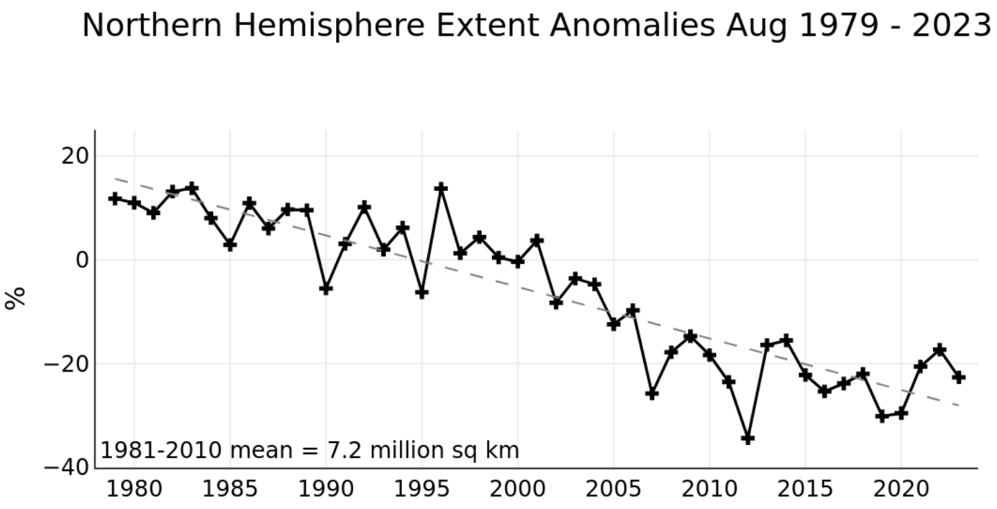
You must be logged in to post a comment.