New Study Debunks Claim That Mid-Latitude Eruptions Cause Extreme Cooling

Explosive volcanic eruptions inject sulfur gases into the stratosphere. These form sulfate aerosols (tiny droplets) that scatter and reflect incoming sunlight back to space, cooling Earth’s surface for months to years. A classic example is the 1815 Mount Tambora eruption in Indonesia, which contributed to the “Year Without a Summer” in 1816.

Extratropical eruptions (roughly mid- latitudes, 30°- 70°) differ from tropical ones mainly in aerosol distribution, lifetime, cooling efficacy per unit sulfur, frequency, and overall climatic influence.

A graphic illustrating two volcanic eruptions, one on the left and one on the right, with the Earth positioned in the background and text overlaying that reads 'New Study Debunks Claim That Mid-Latitude Eruptions Cause Extreme Cooling'.
AI generated by Grok

Explosive volcanic eruptions inject sulfur gases into the stratosphere. These form sulfate aerosols (tiny droplets) that scatter and reflect incoming sunlight back to space, cooling Earth’s surface for months to years. A classic example is the 1815 Mount Tambora eruption in Indonesia, which contributed to the “Year Without a Summer” in 1816.

Dr. Zachary McGraw (Columbia University) and colleagues used a NASA climate model to compare tropical eruptions with extratropical ones (roughly 30°- 70° latitude).

Earlier work had suggested extratropical eruptions produce much stronger Northern Hemisphere cooling, up to about 7.5 times greater for similar sulfur output. The new simulations found only a modest difference at most (up to roughly twice the cooling), with no clear, strong location- based enhancement.

Reasons include:

  • Tropical aerosols are transported into both hemispheres by atmospheric circulation, spreading the reflective cooling more evenly.
  • Extratropical aerosols can stay concentrated in one hemisphere (often the Northern), potentially intensifying local effects, but their overall impact is limited by other factors.
  • Aerosols from extratropical eruptions typically have shorter lifetimes (often up to ~9 months) versus tropical ones (up to ~3 years). This is linked to lower injection heights, removal by precipitation in wetter and cooler mid- latitude conditions, and poleward transport.

When the team compared model results with historical and proxy records (including numerous tropical eruptions after 750 CE), Northern Hemisphere cooling aligned more frequently with tropical eruptions. Extratropical events are rarer and therefore exert less overall influence on Northern Hemisphere temperatures.

In short, the work supports the idea that tropical eruptions play a larger cumulative role in regulating (cooling) Earth’s climate via the “volcanic thermostat” than previously emphasized relative to mid- latitude events. The findings refine understanding of how eruption latitude, season, sulfur amount, and aerosol lifetime shape climatic impacts.

Bar graph comparing the number of tropical eruptions across different datasets: N-TREND, Schneider, LMR Seasonal, and N-scan.
Historical events of cooler-than-normal summers following eruptions in the tropics (top row) and Northern Hemisphere middle latitudes (bottom row). Credit: McGraw et al., 2026.

Extratropical eruptions (roughly mid- latitudes, 30°- 70°) differ from tropical ones mainly in aerosol distribution, lifetime, cooling efficacy per unit sulfur, frequency, and overall climatic influence.

These differences come from the 2026 study by Zachary McGraw and colleagues (summarized in the Phys.org article and detailed in their Geophysical Research Letters paper).

Aerosol distribution and hemispheric effects

  • Sulfate aerosols from extratropical eruptions tend to stay largely confined to the hemisphere of the eruption (often the Northern Hemisphere).
  • Tropical aerosols are transported by stratospheric winds into both hemispheres, spreading the reflective cooling more evenly worldwide.⁠

This confinement can produce some enhanced regional (e.g., Northern Hemisphere extratropical) cooling for extratropical events, but the effect is limited.

Cooling strength

Earlier analyses (including some paleoclimate comparisons) suggested extratropical eruptions could cool the Northern Hemisphere several times more strongly, up to ~7.5 times, than similar- magnitude tropical ones.

Large- ensemble NASA climate model simulations (spanning 5– 40 Tg of stratospheric sulfur, across seasons) found the ratio is consistently only about 1.4- 2 times (typically within a factor of two).

This is explained primarily by the single- hemisphere confinement of aerosols rather than any strongly disproportionate forcing. Paleoclimate evidence (tree rings and historical records) supports similarly modest differences.

Aerosol lifetime

Extratropical aerosols generally have shorter atmospheric lifetimes, often up to ~9 months, versus up to ~3 years for tropical ones.

Contributing factors include:

  • Typically, lower injection heights into the stratosphere.
  • Greater removal by precipitation (rain and snow) in the wetter, cooler mid-latitude climates.
  • Poleward transport of aerosols from mid- latitudes.⁠

Shorter lifetimes limit the duration and cumulative impact of the cooling.

Frequency and cumulative influence

Extratropical eruptions capable of significant stratospheric sulfur injection are comparatively rarer.

As a result, Northern Hemisphere cooling episodes in the historical and proxy record coincide more often with tropical eruptions.

Overall, extratropical events have exerted a smaller cumulative influence on Northern Hemisphere (especially extratropical) temperatures than tropical ones.⁠

In summary, while extratropical eruptions can produce moderately stronger regional cooling due to aerosol confinement, they do not produce the dramatically enhanced effects once claimed, and their shorter lifetimes plus lower frequency mean tropical eruptions play the larger role in Earth’s longer-term volcanic “thermostat.” Effects also depend on exact latitude, season, sulfur mass, and injection height.

No Evidence for Strongly Enhanced Northern Hemisphere Cooling From Extratropical Versus Tropical Eruptions

This open- access research letter directly addresses claims that Northern Hemisphere extratropical (NHET) volcanic eruptions produce several times stronger cooling in the Northern Hemisphere extratropics than tropical eruptions of similar sulfur magnitude.

Key Points

  • Models and tree- ring records show no evidence of greatly enhanced regional cooling from extratropical eruptions versus comparable tropical ones.
  • Extratropical eruptions cool the extratropics no more than is expected from aerosols being confined to one hemisphere.
  • Because large extratropical eruptions are rarer, they have historically caused less overall cooling of the Northern Hemisphere extratropics than tropical eruptions.

Abstract and Main Findings

Prior studies (Toohey et al., 2019; Burke et al., 2023) reported enhancement factors of ~3.2 times or even ~7.5 times for NHET cooling from extratropical versus tropical eruptions.

Using a large ensemble of GISS ModelE2.2 simulations (160 members total) spanning 5- 40 Tg of stratospheric sulfur (VSSI), two seasons (June and December), and locations on the equator versus 64°N, the authors find the extratropical- to- tropical NHET cooling ratio is consistently only 1.4- 1.9 times (within a factor of two).

This matches the physical expectation from aerosol confinement: extratropical aerosols largely remain in one hemisphere, while tropical aerosols spread into both. No additional amplification mechanism is required or supported.

Paleoclimate (tree- ring) evidence yields similarly modest ratios (overall estimates across reconstructions and simulations fall in the 1.4- 2.4 range).

The much larger prior factors are attributed to methodological issues, including reliance on sparse pre- 750 CE data, linear- regression approaches that prove unreliable in synthetic tests, and uncertainties in sulfur and temperature reconstructions for key events (e.g., Laki 1783, 536 CE, Okmok 43 BCE).

Owing to their relative rarity, extratropical eruptions exert a smaller cumulative influence on NHET temperatures than tropical ones. The findings challenge the idea that extratropical eruptions are of outsized importance for Northern Hemisphere climate.

Methods Highlights

  • Prescribed aerosol forcing via a modified Easy Volcanic Aerosol (EVA) framework (adjusted for more realistic shorter lifetimes of summer extratropical aerosols).
  • Interactive ocean and sea ice; NHET temperatures defined as land areas north of 30°N (to match tree-ring coverage).
  • Ensemble approach isolates the forced response from internal variability.
  • The EVA extratropical forcings are shown to be a high estimate of potential cooling relative to interactive aerosol models.

Plain- Language Summary

Volcanic eruptions cool Earth by injecting reflective sulfate aerosols into the stratosphere. Recent claims that mid- to high-latitude eruptions cool the Northern Hemisphere several times more than tropical ones of similar size are not supported.

Climate- model ensembles and temperature reconstructions show at most roughly twice the cooling, exactly what is expected when aerosols stay mostly in one hemisphere.

Large extratropical eruptions are also rarer, so tropical eruptions have had the greater overall impact even on Northern Hemisphere temperatures.⁠

The paper includes supporting information with eruption lists, additional figures on temperature anomalies, regression reliability tests, and tree- ring comparisons.

Full text and SI are available via the DOI or the Columbia-hosted PDF.

Journal: Geophysical Research Letters

DOI: 10.1029/2026GL122071

First published: 15 October 2026

Authors: Zachary McGraw, Benjamin O. Goldman, Lorenzo M. Polvani

Mount Tambora’s 1815 eruption and the year without a summer – Climate- Science.press

The Most Powerful Volcanic Eruptions in Earth’s History

On with the show at UN COP31

So here are a few interesting negotiations to look out for. The beginning of the end of COPs might even be on the table. This is not about the formal agenda because tricky issues have a way of springing up. Surprise is a big part of the spectacle.

First, there is the annual issue of MORE MONEY. Mind you, funding commitments are never mentioned, just more ways to get it. This year there are at least two “funding mechanisms” under discussion.

Cartoon depicting a humorous critique of a climate conference with attendees holding 'Climate Emergency' signs, surrounded by a lavish buffet and a helicopter labeled 'Climate Jet One'.
AI generated by Meta

From CFACT

By David Wojick

COP31 is upon us, and while you may think it is pointless, it is still a spectacle worth watching.

These folks are professional negotiators who could just as easily spend eleven luxury days debating the seating priorities on the first passenger trip to Mars. There is also the enormous global trade show that comes with it.

So here are a few interesting negotiations to look out for. The beginning of the end of COPs might even be on the table. This is not about the formal agenda because tricky issues have a way of springing up. Surprise is a big part of the spectacle.

First, there is the annual issue of MORE MONEY. Mind you, funding commitments are never mentioned, just more ways to get it. This year there are at least two “funding mechanisms” under discussion.

One is called the “Just Transition Mechanism” where the transition is question is the imaginary end of fossil fuel use. The idea is to fund regions, communities, businesses, and people who are hurt by the transition. Unemployed oilfield workers for example, when we stop using oil.

This critter already exists at the EU level having been created around 2021.

The Just Transition Mechanism – European Commission

The issue at COP31 is whether to create a global version of the Just Transition Mechanism.

The second proposed new mechanism is the “Pacific Resilience Facility (PRF),” which is not actually a UN Climate activity. Australia, which just signed a PRF Treaty with Fiji, explains it this way:

“The PRF is the first Pacific-led, owned and managed community resilience financing facility. It will provide grants for climate adaptation, disaster preparedness, and projects that respond to loss and damage. It will seize the economic opportunities of clean energy through resilient, community led projects.”

Australia and Fiji ratify Pacific Resilience Facility Treaty | Australian Minister for Foreign Affairs

What the PRF is doing at COP31 is unclear and there is a lot of that going around.

There are a growing number of non-UN climate activities springing up. Each is driven by the correct observation that the COP extravaganzas are going nowhere.

The leading example is the effort to develop fossil fuel transition “roadmaps” for every country. This is explained in my article “The ‘Transitioning Away from Fossil Fuels’ project has become a global program.”

Another rogue activity is designing a new Fossil Fuel Treaty (FFT) mandating the phase out that countries can adopt (possibly using a roadmap). As a treaty, the FFT would be a legally binding instrument enforceable by the courts. The FFT has its own promoting organization here.

Fossil Fuel Treaty

What is most interesting is that such a treaty has the potential to destabilize the UN Climate Change Program. The UN Program is based on an existing treaty, the 1992 Framework Convention on Climate Change (FCCC). The FFT could compete with the FCCC such as for financial resources and even for jurisdiction. The FFT might even make the FCCC obsolete.

Ironically, the Roadmap rogue started with a suggestion by the COP30 president. The COP31 president has made a new suggestion called the “electrification goal.” The core electrification goal for COP31 is the “35 by 35” pledge, which aims to raise electricity’s share of global final energy consumption from roughly 20–23% today to 35% by 2035. This too may become a non-UN activity.

How COP31 will handle these rogue initiatives is the really big show.

How Farming Triggered Two Medieval Tsunamis in an Italian Lake — And Why the Danger Is Back

Farming and land use helped precondition two medieval lake tsunamis at Lake Iseo (northern Italy), and the hazard has returned because the delta has rebuilt.

Human-induced erosion increases sediment delivery to lake deltas, raising their risk of collapse. At Lake Iseo, roughly two millennia of intensified land use (deforestation, agriculture, pastoralism) tripled sediment flux to the lake. This over steepened the Oglio River delta and preconditioned it for failure.

A dramatic landscape featuring a mountainous region with terraced farming, facing an immense tidal wave crashing towards the shores, under a cloudy sky with rays of sunlight piercing through.
AI generated by Grok

Farming and land use helped precondition two medieval lake tsunamis at Lake Iseo (northern Italy), and the hazard has returned because the delta has rebuilt.

This is based on a 2026 Nature Communications paper (“Human- enhanced tsunami hazard in large lakes”) led by Muhammad Naveed Zafar, with co-authors including Denys Dutykh (who wrote the Phys.org piece summarizing the work). The team combined sediment cores, seismic profiles, historical and archaeological evidence, and numerical modeling of landslides and waves.

Lake Iseo sits at the foot of Val Camonica in the southern Alps. The Oglio River builds a large delta at its northern end. Since Roman times, forest clearing, farming, and grazing in the catchment have tripled sediment delivery to the lake relative to earlier Holocene levels.

This rapidly built up and over steepened the underwater delta front, making it unstable. A prior collapse had already occurred in the 6th century; centuries of accelerated erosion then reloaded it.

The two events

  • 3 January 1117: A magnitude ~6.5 earthquake (near Verona) triggered collapse of ~62 million m³ of sediment. Simulations show waves reaching northern shores in under a minute, with run- ups of ~50 m near the delta and flooding up to ~2.7 km inland along the Oglio plain. Farther south (e.g., at Iseo town), run-up was ~5.5 m after 6- 7 minutes. Monte Isola partly sheltered southern shores. A contemporary Vatican Library manuscript notes lakes rising so high that few nearby villagers escaped.⁠
  • Christmas Day 1222: A magnitude ~6.0 earthquake triggered a smaller collapse (~10 million m³) after the river had partially rebuilt the front. Modeled run- ups reached ~13 m.⁠

The thickest mass- wasting deposits in the deep basin (up to ~250 m depth) match these volumes and locations. Modeling treated the slides as viscoplastic mud and the long waves with shallow-water equations (waves traveled ~50 m/s or ~180 km/h in deep water). Results align with historical accounts, church rebuilds, archaeological damage, and the absence of deposits in sheltered southern areas.

After 1222, land- use pressure eased temporarily (e.g., during the Black Death) but intensified again from the 17th century and peaked in the industrial era. Eight centuries of continued human- driven erosion has rebuilt the delta front. Lake Iseo’s shores are now densely populated. A similar collapse today would reach northern towns (e.g., Pisogne, Lovere) in seconds to under a minute, too fast for effective warning in many places, with more time (minutes) farther south.⁠

Similar human- amplified risks exist elsewhere (e.g., evidence of medieval collapses in Lakes Garda and Como; analogous cases from Lake Geneva to Alaska and New Zealand). Global sediment delivery to lake deltas has risen sharply with modern land use, increasing the potential for future failures.⁠

In short, people did not cause the earthquakes, but centuries of farming and deforestation overloaded the delta, turning seismic shaking into catastrophic underwater landslides and tsunamis. The same process has reset the hazard.

Map of Lake Iseo at the foot of Val Camonica, highlighting its delta, deep basin, and historical seismic events in 1117 and 1222.
Lake Iseo lies at the foot of Val Camonica, in the southern Alps of northern Italy, where the Oglio River enters it from the north and has built a delta. The two stars mark the earthquakes of 1117, of magnitude 6.5, and of 1222, of magnitude about 6. On the map of the lake (right), the darker the water, the deeper the lake, down to 250 meters in the long northern basin; the dark red line outlines the front of the delta that collapsed in 1117, and the orange dashed line the part that collapsed in 1222. Credit: Denys Dutykh; data: Zafar et al. 2026 (Figshare, CC BY 4.0), Terrain Tiles (AWS Open Data), Natural Earth, CPTI15 catalog (INGV)

Lake Iseo tsunami modeling methods (from Zafar et al., Nature Communications 2026) used a one- way coupled two- stage approach: first simulate the subaqueous landslide dynamics, then feed the resulting time- dependent bathymetric changes into a tsunami propagation, inundation model. Feedback from the waves onto the landslide is neglected, but hydrodynamic forces (viscous drag, added mass) are included in the landslide stage.

1. Reconstruction of pre- failure geometry and volumes

  • High-resolution LiDAR topography and multibeam bathymetry (2002 surveys by Regione Lombardia and OGS, CARG program).
  • Present- day bathymetry served as a morphological analogue for the pre-failure delta (assuming post- event sedimentation largely infilled the scars along a similar pathway).
  • In GIS, post- failure morphology was reconstructed by removing accumulated sediment and restoring a plausible failure- scar shape guided by bathymetric trends and erosional features.
  • Source volumes were calculated as the difference between the reconstructed post- failure surface and modern bathymetry, then iteratively adjusted until they matched the volumes of the mapped mass-wasting deposits (from seismic profiles + sediment cores) in the deep basin:
    • 1117 CE: 6.2×1076.2×107 m³
    • 1222 CE: 1.0×1071.0×107 m³
  • Assumption of single- event failure supported by the sedimentology of the deposits (erosive sandy base → single upward-fining unit → homogeneous suspension- settling layer from seiches).

2. Landslide modeling (BingClaw)

  • Two- layer, depth- averaged (2HD) viscoplastic debris- flow model BingClaw.
  • Rheology: Herschel- Bulkley (suitable for cohesive subaqueous landslides).
  • Layers:
    • Upper plug layer (moves en bloc, no internal shear).
    • Lower shear layer (deforms once shear stress exceeds yield strength).
  • Mass balance solved over the full depth; momentum equations solved separately per layer with a Godunov- type finite- volume scheme.
  • Key rheological parameters chosen to best match observed runout distance, deposit thickness, and spatial distribution (runout is most sensitive to yield strength):
    • 1117 CE: yield strength 25 Pa, bulk density 1600 kg m⁻³
    • 1222 CE: yield strength 7 Pa, bulk density 1650 kg m⁻³ (lower yield strength reflects higher water content and coarser sediment fraction)
    • Other fixed parameters (from literature and validation studies): fluidity index n=0.5n=0.5, added mass 0.1, frictional drag 0.01, pressure force 1.0, reference strain rate 100 s⁻¹.
  • Output: time- evolving landslide thickness and runout until final deposition in the deep basin (validated against seismic profiles and cores). The 1222 CE slide traveled farther and faster due to lower strength and more accommodation space.

3. Tsunami modeling (GeoClaw)

  • Time-dependent bathymetric changes from BingClaw drive wave generation.
  • Model: GeoClaw: 2- D depth -averaged nonlinear shallow- water equations (NSWE).
  • Features: shock- capturing Godunov- type finite- volume scheme, adaptive mesh refinement, effective wet or dry interface handling for inundation.
  • Grid resolution: ~10 m rectangular cells.
  • Manning roughness coefficient: 0.03.
  • Lake level: modern reference (185.44 m a.s.l.); no significant level change inferred over the last ~2 kyr.
  • Waves are long (~5.5 km wavelength for 1117 CE, ~22× maximum lake depth of 250 m), so NSWE is appropriate; water moves nearly as a coherent sheet.
  • Long- wave speed ≈gh≈50≈gh​≈50 m s⁻¹ (~180 km h⁻¹) in deep water.

4. Additional analyses and sensitivity

  • Froude number (Fr=U/gh​, where U is landslide velocity magnitude): calculated to assess generation efficiency (most efficient near Fr≈1Fr≈1). Tracked temporally for the 1117 CE event.
  • Dispersion sensitivity: comparison of nondispersive NSWE vs. a more complete (Boussinesq- type) model; results were nearly identical at the same times, supporting the NSWE approximation for these long waves.
  • Initiation- depth sensitivity: alternative scenarios with the 1117 CE failure starting deeper (45 m or 75 m below surface) produced lower maximum run-ups (~22 m or ~11 m instead of >50 m).
  • Validation: modeled deposit geometries match observations; tsunami results consistent with historical accounts (Vatican manuscript), archaeological damage (e.g., church of Sant’Andrea), and absence of deposits in sheltered southern areas.

Simulations used the Clawpack framework (BingClaw and GeoClaw).

Simulation data (outputs, Makefiles, plotting scripts for both events, including optional Boussinesq runs for 1117 CE) are available on Figshare. The approach has been validated on other events (e.g., Storegga, Alpine lake slides).

These methods combine geological constraints with physics- based numerical modeling to reconstruct the two medieval events and assess modern hazard.

A schematic cross-section illustrating the delta of the Oglio river to Lake Iseo, showing different phases: before Roman times with a forested delta, an overloaded delta due to land use, consequences of an earthquake lifting water and causing waves, and the delta regrowth over eight centuries.
How human land use caused the collapses, in a cross-section of the delta from the mouth of the river to the deep basin (a schematic, not to scale). Before Roman times, forested slopes fed the delta at a lower rate. Over 2,000 years, forest clearing, farming and grazing tripled the sediment reaching the lake, and the front of the delta grew steep and overloaded. An earthquake shook the front loose: the mass slid into the deep basin, the water dropped above the scar and rose ahead of the slide, and waves ran out across the lake and back onto the nearby shores. Today the two collapses lie buried as thick layers in the deep basin, where cores find them, and the front has grown back. Credit: Denys Dutykh

Human-enhanced tsunami hazard in large lakes

Human-induced erosion increases sediment delivery to lake deltas, raising their risk of collapse. At Lake Iseo (northern Italy), roughly two millennia of intensified land use (deforestation, agriculture, pastoralism) tripled sediment flux to the lake. This over steepened the Oglio River delta and preconditioned it for failure.

Geological records and numerical simulations show that earthquakes in 1117 CE (Mw 6.5) and 1222 CE (Mw 6.0) triggered major subaqueous delta collapses.

These generated tsunamis with maximum run- ups of approximately 50 m and 13 m, respectively. Historical accounts (Vatican Library manuscript) and archaeological evidence support the reconstructions.

Since the last collapse, eight centuries of continued human- driven erosion has rebuilt the delta. Shoreline populations are now highly vulnerable to future earthquake- triggered failures.

A global lake synthesis indicates that human- driven erosion has reached its highest levels since the Industrial Era, progressively overloading delta’s worldwide and potentially increasing the likelihood of similar events.

Main Results from Lake Iseo

  • Sediment loading: Since Roman times, human activities tripled sediment flux relative to earlier Holocene background levels. The delta front became steep and overloaded. A prior collapse occurred in the 6th century; further accumulation reloaded it.
  • Collapse volumes:
    • 1117 CE: ~62 × 10⁶ m³ (thickest deposit ~7 m in the deep basin).
    • 1222 CE: ~10 × 10⁶ m³ (deposit ~2 m thick), after rapid rebuilding in the intervening century.
  • Tsunami modeling:
    • 1117 CE: Waves >50 m near the northern shores; reached shores within ~1 minute; inundation up to ~2.7 km inland along the Oglio plain. At the town of Iseo (~7 min later), ~5.5 m run- up. Monte Isola partially sheltered southern areas.
    • 1222 CE: Peak waves ~13 m; inundation up to ~1 km inland.
  • Validation used sediment cores, seismic profiles, viscoplastic landslide modeling, and nonlinear hydrodynamic (shallow- water) tsunami simulations. Results match deposit geometries and historical and archaeological evidence (e.g., damage and rebuilding of the church of Sant’Andrea in Iseo; minimal impact and no deposits in the sheltered southern Torbiere del Sebino area).

The work demonstrates a persistent, human- amplified mechanism for generating large lacustrine tsunamis. Similar overloaded deltas and thick mass- wasting deposits exist in other lakes (e.g., Garda, Como).

Modern high sediment delivery rates mean comparable failures may become more likely under seismic loading. Hazard assessments for densely populated lake shores in tectonically active regions should incorporate long- term anthropogenic sediment dynamics, not only seismic sources.⁠

The paper integrates geophysics, sedimentology, history, archaeology, and numerical modeling (landslide rheology and tsunami propagation and inundation). Supplementary materials include cores, seismic profiles, and additional figures.

Corresponding author: Muhammad Naveed Zafar.

Infographic illustrating the collapse of 1117 in a landslide model, showing five stages: initial state, after 1 minute, after 3 minutes, after 10 minutes, and after 50 minutes, with annotations for delta front volume and thickness of the sliding mass.
The collapse of 1117 in the landslide model, from its start to 50 minutes later. At the start, a crescent of sediment holding 62 million cubic meters sits on the front of the delta. The mud stays rigid until it is pushed beyond its yield strength, then flows: after 1 and 3 minutes it pours down the slope, after 10 minutes it runs along the deep basin, and after 50 minutes it rests there as a layer about 5 meters thick, more than 10 kilometers from where it started. Credit: Denys Dutykh; data: Zafar et al. 2026 (Figshare, CC BY 4.0), Terrain Tiles (AWS Open Data)

Journal: Nature Communications, volume 17, Article number: 10531 (2026)

DOI: 10.1038/s41467-026-78272-8

Published: 15 October 2026

Authors: Muhammad Naveed Zafar,
Pierre Sabatier,
Denys Dutykh,
William Rapuc,
Raphaël Paris,
Andrea Piccin,
Pascal Vuillemin &
Flavio S. Anselmetti

Abstract

Worldwide, human-induced erosion enhances sediment delivery to lake deltas, increasing their susceptibility to collapse. In Lake Iseo, northern Italy, two millennia of intensified land use tripled sediment flux, oversteepening the delta and preconditioning it for failure. Here we show from geological records and numerical simulations that earthquakes in 1117 CE (Mw 6.5) and 1222 CE (Mw 6.0) triggered major subaqueous delta collapses, generating massive tsunamis with maximum run-ups of ~50 m and ~13 m, respectively. Historical accounts from the Vatican Library and archeological evidence support these reconstructions. Since the last collapse, eight centuries of human-induced erosion have rebuilt the delta, leaving shoreline populations highly vulnerable to future earthquake-triggered failures. A global lake synthesis showed that human-driven erosion has reached its highest levels since the Industrial Era, progressively overloading deltas worldwide; thus, similar catastrophic failures may become more likely in the future. These findings reveal a persistent, human-amplified mechanism of lacustrine tsunami generation and intensity with major implications for hazard assessment.

An ominous “Sandyversary”

With the anniversary of Sandy, I wanted to show the evolution of our forecasts. I had Grok look at all our issuances from Oct 22, and I had it issued a summary of what was out in public the 25th. Our first warning went out the 21st. And references to past events explaining how a storm like this should happen and is natural were also shown.
Bastardi published this on Thursday, October 25, 2012, while the system that became Hurricane Sandy was still developing in the Caribbean/Atlantic (around the time it was named or shortly after). He and WeatherBELL had already been issuing client warnings since the previous weekend. The piece is both a forecast update and a longer-term argument about why this kind of event was expected.

A dramatic depiction of Hurricane Sandy over a coastal area, with dark storm clouds and lightning, and the text 'Sandyversary' prominently displayed.
AI generated by Meta

From CFACT

By Joe Bastardi

Satellite image showing a large storm system impacting the southeastern United States, with cloud formations and weather patterns visible.

With the anniversary of Sandy, I wanted to show the evolution of our forecasts. I had Grok look at all our issuances from  Oct 22, and I had it issued a summary of what was out in public the 25th. Our first warning went out the 21st.  And references to past events explaining how a storm like this should happen and is natural were also shown.

AI summary of a public post on the 25th:

Context and timing

Bastardi published this on Thursday, October 25, 2012, while the system that became Hurricane Sandy was still developing in the Caribbean/Atlantic (around the time it was named or shortly after). He and WeatherBELL had already been issuing client warnings since the previous weekend. The piece is both a forecast update and a longer-term argument about why this kind of event was expected.

Core forecast and warnings
Bastardi states he had been “loudly warning” WeatherBELL clients of a historic storm in the making.
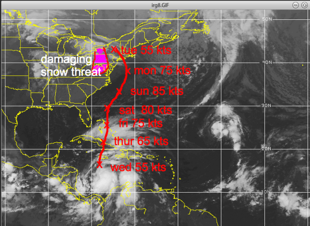
On the Sunday before the column, they put out a chart showing the system (still unnamed at that point) hitting near New York City from the south-southeast as a 75-knot hurricane early the following week.
By October 25, he had adjusted his forecast slightly south: landfall into New Jersey, with a major snowstorm on the western side from western Pennsylvania into West Virginia.
He described it to clients as a multibillion-dollar storm where it hit, and potentially the worst historically in some Mid-Atlantic coastal areas. He noted the window for it to miss was closing.
The “Philadelphia Story” scenario
Bastardi had long wondered why a hurricane from the southeast had never struck the mid- or northern Atlantic coast ( my dads idea). He routinely illustrated this in talks as the “Philadelphia Story”:

A hurricane approaches the Mid-Atlantic from the southeast, near or south of the mouth of Delaware Bay.
It drives a storm surge up the funnel-shaped Delaware Bay (analogous to what the 1938 hurricane did in Providence).
That surge meets river flooding coming downstream on the Delaware River (worsened by modern dam releases from upstream lakes).
Such a storm would also devastate the Jersey Shore worse than the 1944 hurricane.
He framed the developing event as the combination of individual past events coming together in one place. Rather than asking “why is this happening?”, he said he had always wondered “why hasn’t this happened yet?”

Seasonal and pattern context
WeatherBELL had said from the start of the 2012 hurricane season that the end of the season would feature a tropical cyclone coming out of the Caribbean and threatening the East Coast.
They expected an end-of-season pattern similar to the in-close storms that opened the season.
Three weeks earlier, they had again told clients the pattern was setting up for this.
Natural causes, not global warming
Bastardi repeatedly stressed that the storm would result from natural atmospheric processes and pattern recognition, not man-made global warming or CO2:

A tropical cyclone interacting with a massive early-season cold air mass, forcing a northwest turn into the Mid-Atlantic.
Historical precedents: his father (a degreed meteorologist) used to show him hurricane tracks and note that shifting a track by only a couple of hundred miles would produce exactly this kind of outcome. Meteorologists had recognized the setup as possible for years.
“It will not be global warming but the combination of natural events that will cause it… If it does occur, it will be because of nature, not man.”
Closing
He invited readers to WeatherBELL.com for detailed tracking (including a trial option and access to prior archives showing how long they had been setting the event up). He ended by describing the weather as “a majestic display of creation” that humans cannot control but can observe and try to understand.

Later references
Bastardi later cited this exact October 25 column (and the earlier client warnings starting around October 21) in subsequent Patriot Post pieces as evidence that Sandy was a forecastable, pattern-driven event rather than an unprecedented CO2-linked disaster. He contrasted the early WeatherBELL guidance with more delayed or different official outlooks at the time.?

This is a concise but complete rendering of the article’s content and argument.

So here are those updates (just the maps of our tracks):

October 22nd WeatherBELL Analytics Tropical Update

October 22,2012

Right off the bat, here is the latest idea: very close to yesterday and it is the “capturing” (ECMWF) rather than escape scenario, as per the GFS.

Satellite image showing weather patterns over the eastern United States and Caribbean, with annotated wind speeds in knots for various days of the week.

I  think the capture is most likely . The “Wilma” idea of a storm is out, but new strong, non-tropical is second, and the total escape is last.

October 23rd WeatherBELL Analytics Tropical Update:

October 23, 2012

Weather radar image showing tropical system predictions with wind speeds in knots for each day of the week, highlighting a 'damaging snow threat' in the northeastern United States.

A damaging snowstorm is possible to the west of the track of this early next week in the mountains.

October 24, 2012

I have no changes in the reasoning on Sandy. The forecast if a blend of the ECMWF operational and yesterday’s idea. I will cut right to the point.

Satellite image showing weather forecasts including a damaging snow threat in the northeastern US, with wind speed estimates for several days labeled in red, and the path of Hurricane Tony indicated.

The idea remains the same: the escape is the least likely, the Wilma (storm out to sea but nor’easter develops) is second, and the most likely for the reasons I have been laying out since Sunday, being the track we have now.

October 25th WeatherBELL Analytics Tropical Update

October 25, 2012

I am well aware of all the different model ideas, but my ideas on this remain the same with the forecast representing the capture option as it has from Sunday. I still list the total escape idea, but it is now 1 in 10 chance. The Wilma option remains a 3 in 10 chance, which means my idea is now 3 in 5, if we are looking at this from the idea of all 3. One has to make a forecast though, so the forecast remains the same.

Satellite image showing a weather map with a focus on a winter storm threat in the northeastern United States, along with wind speed predictions for various days of the week.

Keep in mind when this was put out the NHC track was this:

Weather map showing the projected path of a hurricane with time markers and locations, including Bermuda and parts of the southeastern United States.

And there were other forecasts still having a complete miss.

The implication here is for a 10–20-billion-dollar storm, and the threat of a major disaster for the ports of PHL and ILG should the center go ashore and shove the storm surge up the Delaware Bay and flooding coming down the river. This has been something I have written on over the years, asking myself why it has not happened. Also devastated to the maximum degree would be Atlantic City as their beach faces south-southeast and is cup shaped. All the coast from Hatteras north would have hurricane winds and unlike Irene, which weakened, this would spread out true, but the baroclinic support would simply make her as powerful over a larger area rather than focused fury at the center. This will use non tropical energy sources to max out over the water, which is very much above normal.

To be blunt, it is the focusing of low level heat from the warm ocean in the very area that the coldest deviations from normal aloft are going to occur. Until nature can do her job and balance it out, the storm will deepen, then release. Crushing snows measured in feet will fall from western Pennsylvania into West Virginia, and snow may even reach secondary cities from Roanoke to Harrisburg, perhaps even into DC by the end.

Landfall Monday was at 935 mb before the weakening started.

October 26th WeatherBELL Analytics Tropical Update

October 26, 2012

I have merely adjusted the previous track a bit and the forecast is a blend of the old track, ECMWF and GFDL. The storm will re-intensify tomorrow and Sunday as it gets away from the upper feature that has captured it now. The question, of course, is where will the turn back be? I believe the ECMWF is the closest model and the landfall is half way between my idea yesterday and its 00z run, which the GFDL looks a lot like.

The “pick your poison” option is focused most heavily on the Delmarva, NJ and the threat of the major surge up Delaware Bay compounded by the river water rushing down, which could put the ports of PHL and ILG in a very bad position. A 10-15 foot storm surge is possible with this, which would inundate the coast in a way not seen since 1944 (it would probably be worse). The old GFS, if correct with the hit further north and the driving of water down the Long Island Sound while the storm surge tries to advance west, would mean NYC would have record high water. Such an event could put tunnels and subways under water. Again, pick your poison, since it seems the escape route east of the storm is out.

Given foliage still on trees, power outages equal or greater to Irene and a damage total similar or greater seems to be likely. The heavy snow area may be paralyzed for a few days, and is shown in purple.

Satellite image depicting weather patterns with storm tracks, wind speeds, and potential landfall locations, including storm surge estimates.

Special Sandy Update – October 27, 2012

October 27, 2012

Sandy at 967 mb rates about 3.75 out of 10 on my scale, still a hurricane. The recon has 63 kt surface winds and how a storm is downgraded with that pressure and the plane finding that surface wind without flying over every single square inch of the storm is a classroom exercise, not a realistic approach. The power scale showed its mettle in Isaac and with Sandy as the storms “tighten” coming to land. Sandy will always have less wind, given her pressure, than a hurricane in the tropics. But with a favorable outflow and jet entrance region developing the rest of the way in, and water as high as 28c, this is going to re-deepen, in my opinion, to at least 950, probably close to 940.

The latest track takes her inland on the central Jersey coast, north of the major disaster path for PHL but very close to the path that could lead to a devastation of Atlantic City (landfall just south). This path is also very close to the path that would lead to the unthinkable in NYC, such as has been shown at hurricane conferences, enough of a surge to put a large part of NYC underwater as sound side flooding and Atlantic storm surge combine. I have gone over all these options; the path is in the middle of what is now a 7-day spread of paths that started Sunday.

Satellite image showing a weather system over the southeastern United States with wind speed measurements and forecasted landfall details.

October 28, 2012

This storm will be everything said about it, and more. On my scale with pressure in mid Category 3 and wind 90% of flight level, this is a 4.85 out of 10. Its pressure is around Ike’s already and in fact, one could say this is the Northeast equal to the Ike situation, a storm that will do far more damage than what its category implies.

Naturally, I think NHC not issuing hurricane warnings and playing classification games is folly. Those things should be left for hurricane conferences, not here. But that is all I wish to say on that matter.

The track is in the mid ground of what is now an 8 day forecast period that has been given to you.

Look for the pressure to bounce up and down until the convection can get wrapped around again, but the overall idea of the intensification trend that I am expecting to see today into tomorrow appears to be starting.

Satellite image showing a weather map of the eastern United States with a tropical storm highlighted, including wind speeds and pressure readings for specific days.

October 29, 2012

Notice back in 2012 how much size mattered.

Sandy is now rated 5.1 out of 10 on my power scale, which gives barometric pressure equal weight in assessing the storms overall capability. This idea is because the lower the pressure, even though the wind may not be in one spot, the more overall power the storm has and it also helps determine whether the storm could tighten up and wind increase as we are seeing now with Sandy. For reference, Katrina was 8.3, Ike 5.5. Last year, Irene (when it reached the Northeast) was a 4, as was Isaac this year. This is about as severe a situation as we can imagine for the Northeast areas from Delmarva to Long Island with a landfalling storm as described in the map below near Atlantic City this evening, or very close to the cumulative midpoint of WeatherBell ideas since last Sunday.

Satellite image showing weather patterns with markers indicating wind speeds and pressure at different times during a storm's approach and landfall.

Note The pressure  was 945.5 at Somers Point NJ when the eye passed. Strongest winds came from the south after the eye passage. The witness was a degreed meteorologist ( my dad) who has been in 7 hurricanes, 3 of them that passed right over him in Rhode Island ( 38,44,54. He said those had nothing on Sandy

15-30 inch snows will blanket from northern North Carolina to the West Virginia mountains, though most low areas will have much less. Backlash wet flakes may make it in to DC and BWI. The snow is pretty much as outlined last week.

I expect NHC to have to up this as it comes to land and the storm surge map will have to add another layer (13-15 feet). Keep in mind the power rating from Friday was the reason I said this would have a 10-15 foot surge.

A map showing the northeastern United States, highlighting New York, New Jersey, Pennsylvania, Connecticut, and surrounding areas.

There isn’t much more to say here that hasn’t been said before, except that the hurricane season ended the way it started and we opined about, in close and with warmer water, the threat of a bigger hit. The MJO rolled right into where one wanted to see it for this and strong amplitude of 1 to 2 was a hint this could happen well in advance. One of the benefits of being the son of a hurricane studying meteorologist (my dad) was that I saw so many maps of storms that could have done what this did, but were further west, that when the set up came, I recognized at least the threat.

In any case, I think we can agree this was not a hype storm, but will live up to its billing.

This should shut down the hurricane season, but again you must balance out what I have forecasted as far as the sensible weather with the power outage implication vs the cold. This will cause more damage than Irene.

October 30, 2012

Sandy will wind down over the northeast the next few days and with the MJO moving away from its favored phases for development in the late season, the end game storm out of the western Caribbean is most likely to be just that.

The tropics should be quiet the next several days (weeks, months probably).

Obviously, I will keep my eyes open.

And ominous Sandyversary.  A storm 30-50 miles further south; it is the Philadelphia story. And sometimes that track should happen also.  And it will have nothing to do with climate man made climate change, and everything to do what nature was made to do.

Germany Enters Winter with Record-Low Gas Storage, Raising Price and Supply Risks

German gas storage is currently low for the start of the heating season.
EU- wide storage is higher at around 74- 75%
The low German gas storage levels (around 61% at the start of the heating season, missing the ~70% target) primarily create risks of higher energy prices and reduced buffers rather than an immediate supply crisis.
If German (or broader European) gas storage levels drop below 50% during winter, the system becomes significantly more vulnerable, though it does not automatically mean an immediate physical shortage or blackouts.

Infographic showing Germany's natural gas storage levels in January 2024, highlighting critical low storage at 18.7%, with indicators of supply risks and rising gas prices.
AI generated by Grok

German gas storage is currently low for the start of the heating season.

As of late October, and 1 November 2026, levels stand at roughly 61- 61.6% full (around 151- 152 TWh of working gas out of ~247 TWh capacity), according to AGSI+ data reported by sources including the Bundesnetzagentur, gasspeicherkarte.de, and multiple news outlets.

This missed the national target of about 70% by 1 November (most sites aim for 80%, with some exceptions at 45%, averaging ~70%). It is well below the five-year seasonal average (historically closer to 85- 90% and more at this time of year) and the lowest on record for late October and early November in available data going back to 2011.

EU- wide storage is higher at around 74- 75%.

Official view vs. industry warnings

  • The Bundesnetzagentur (Federal Network Agency) and Economy Ministry state that supply remains secure and the risk of a strained situation is low. They emphasize that storage is only one factor; ongoing pipeline imports (especially from Norway), LNG terminals, European interconnectors, and demand management matter more. They note that traders handle much of the winter hedging and that missing the exact target is not automatically critical. State-owned SEFE has been directed to add more gas.⁠
  • The storage industry association INES calls the shortfall a “serious warning”. Germany is entering winter with smaller safety buffers and could be more vulnerable to prolonged extreme cold or import disruptions. They have urged stronger measures for future winters.

Prices have been elevated (TTF around €100 and more /MWh recently in some reports), influenced by global factors including the Iran- related disruptions, which complicated summer refilling.

Weather context

Temperatures are dropping seasonally, with frost already occurring in places and forecasts pointing to cooler conditions and possible colder air (including polar and continental influences) around mid- November.

This will increase heating demand and accelerate storage withdrawals, which have already begun in net terms. Long- range signals remain uncertain, but early cold spells would test the lower starting stocks.

Bottom line: Levels are uncomfortably low by historical and target standards heading into winter, reducing the cushion against a hard winter. Authorities are not sounding alarms about shortages under normal- to- moderate conditions thanks to diversified imports, but the margin for error is thinner than in recent high- storage years. Monitoring daily AGSI+ and Bundesnetzagentur updates and weather will be key over the coming weeks.

Graphic displaying the gas storage tank levels in Germany and Europe as of October 31, 2026, highlighting percentage levels and comparisons with previous days.
Gas storage filling level currently: 61.0 % in Germany

The low German gas storage levels (around 61% at the start of the heating season, missing the ~70% target) primarily create risks of higher energy prices and reduced buffers rather than an immediate supply crisis.

Authorities (Bundesnetzagentur and the Economy Ministry) assess the risk of strained supply as low under normal conditions, thanks to diversified imports (Norway pipelines, LNG terminals, European neighbors).

However, the thinner cushion amplifies vulnerabilities, especially for energy-intensive industry and households.

Key economic impacts

  • Higher and more volatile gas and electricity prices: European TTF prices have already roughly tripled this year (hitting levels above €100/MWh at times, the highest since late 2022), driven mainly by the Iran- related disruptions to global LNG, shipping but worsened by lower European (especially German) stocks. This forces greater reliance on spot-market purchases. Wholesale costs feed into household heating bills and industrial energy expenses. New household gas tariffs have risen (e.g., reports of averages around 11- 14 ct/kWh range recently), and network fees have also increased. A cold snap or further supply tightness could push prices higher, adding to cost- of- living pressures.⁠
  • Pressure on industry and competitiveness: Germany’s energy- intensive sectors (chemicals, steel, manufacturing, pharmaceuticals, mechanical engineering) are particularly exposed. High or spiking gas power prices raise production costs, squeeze margins, and can force output cuts if prices exceed affordability thresholds during cold peaks. Industry groups have warned of potential significant economic damage in a very cold winter with low stocks. This compounds existing competitiveness challenges from elevated energy costs post- Russia gas phase- out. Some analysts note that low stocks increase exposure to global LNG markets, where Europe competes with Asia.⁠
  • Inflation and broader growth effects: Elevated gas prices tend to pass through to broader inflation (energy is a key component of HICP/CPI). One modeling estimate suggested a sustained high TTF level could add modestly to peak inflation. Higher costs reduce real household incomes and industrial investment, weighing on GDP growth in an already challenged German economy. Extreme scenarios (prolonged cold and import disruptions) could lead to demand rationing or voluntary cutbacks with larger output losses; milder winters keep effects mostly price- driven.
  • Household burden: Higher heating costs hit consumers directly. Regulators have explicitly warned that gas has become “considerably more expensive” and customers should prepare for this. Lower- income households face greater relative impact, potentially increasing social and political pressure.
  • Spillover to the rest of the EU: As Europe’s largest gas consumer and storage holder, Germany’s extra winter buying can tighten the continental market and lift prices elsewhere (Italy has publicly criticized Berlin on this point).

Mitigating factors and outlook

Diversified supply routes, LNG capacity, and ongoing imports reduce the chance of physical shortages in an average winter. The government has ordered extra purchases via SEFE and is discussing stronger storage obligations for future seasons. Storage deliverability (withdrawal rates drop as levels fall) becomes more relevant late in a hard winter (e.g., February- March).

Overall: The main near- term economic hit is through sustained higher energy prices rather than blackouts or widespread rationing. This adds headwinds to inflation control, industrial competitiveness, and household purchasing power. A mild winter limits the damage; a cold one with continued global tightness would amplify costs and risks for Germany’s manufacturing- heavy economy. Monitoring weather, LNG flows, and daily storage draws will determine how severe the effects become.

Line graph displaying natural gas prices in EUR/MWh from January 2022 to September 2023, showing fluctuating trends with highlighted price peaks and lows for the Day Ahead and Future market indicators.
Federal Network Agency – Current situation Gas supply – Gas prices wholesale in EUR/MWh

If German (or broader European) gas storIf German (or broader European) gas storage levels drop below 50% during winter, the system becomes significantly more vulnerable, though it does not automatically mean an immediate physical shortage or blackouts.age levels drop below 50% during winter, the system becomes significantly more vulnerable, though it does not automatically mean an immediate physical shortage or blackouts.

Effects depend heavily on the timing (early vs. late winter), weather severity, ongoing import rates (pipelines and LNG), and demand.

Technical and operational effects

  • Reduced deliverability (withdrawal rates): As fill levels fall, reservoir pressure drops. Storage sites cannot withdraw gas as quickly. On peak cold days, storage can normally cover a large share of demand (sometimes >50% in extreme conditions). Below ~50% (and especially lower), the maximum daily output declines, making it harder to meet sudden spikes even if gas remains in the ground.⁠
  • Smaller seasonal buffer: Storage typically supplies a substantial portion of winter demand. Crossing below 50% earlier than usual leaves less reserve for the rest of the season, especially late winter (February- March), when the legal German target is only 30% (40% for some Bavarian sites).
  • Higher risk of shortfalls in extreme scenarios: Industry modeling (e.g., by INES) shows that even starting the winter at ~77% can lead to daily shortfalls of >25% under extreme cold. Starting lower or dropping below 50% mid- winter amplifies this. In very cold conditions with constrained imports, temporary supply gaps become more likely.

Market and price effects

  • Sharper price spikes: Markets react quickly to tighter inventories. Wholesale gas prices (TTF) would likely rise further as traders bid more aggressively for remaining LNG cargoes and pipeline volumes. This feeds into electricity prices (gas often sets the marginal power price). Household and industrial bills would rise with a lag.
  • Greater reliance on spot markets and imports: Germany would need to import more on a day- to- day basis, competing with Asia and other European buyers. Any LNG disruptions (e.g., weather, geopolitics) hit harder.

Economic and supply- security consequences

  • Industry first in line for restrictions: Protected consumers (households, hospitals, critical infrastructure, some combined heat- and -power plants) have priority. In a genuine shortage (“Gasmangellage”), the Bundesnetzagentur can order industrial demand reduction or curtailment to protect households. Energy- intensive sectors (chemicals, steel, manufacturing) would face higher costs or forced output cuts first.
  • Broader economic pressure: Higher energy costs raise inflation, squeeze industrial competitiveness and margins, and reduce household purchasing power. Extreme cases could lead to measurable GDP impacts via production losses.
  • Knock- on to the power system: More expensive or constrained gas raises electricity prices and can stress the grid if gas- fired plants are needed for balancing (especially during low wind and solar periods).

Context and thresholds

Germany’s current starting level (~61%) already provides a thinner cushion than in recent high- storage years. Officials currently rate the risk of a strained situation as low for an average winter because of diversified imports.

However, dropping below 50% (particularly if it happens relatively early or coincides with a cold snap) would increase the probability of tighter conditions and higher prices.

Historical winters have seen levels fall well below 50% (even toward 20%) by late winter without collapse when imports held up, but those started from much fuller autumn positions.

In short: Below 50% does not equal empty tanks or widespread rationing under normal conditions, but it shrinks the safety margin, slows peak withdrawal capability, raises the chance of price spikes or temporary industrial restrictions in cold weather, and leaves less buffer for the following season.

Continuous imports and demand management remain the key mitigants. Real-time monitoring of weather, LNG arrivals, and daily storage draws would determine the exact outcome.

Infographic showing gas storage levels in Germany at 61.03%, labeled as "Critical" due to being the lowest level in the past ten years on this date. It includes comparisons to previous day, last year, and historical data from 2016 to 2025.
Germany gas storage levels today: 61.0% (Critical)

Gas storage levels in various European countries, showing percentages and status (Comfortable, Normal, Below average, Tight, Critical).
Germany gas storage levels today: 61.0% (Critical)