Global warming, climate change, all these things are just a dream come true for politicians. I deal with evidence and not with frightening computer models because the seeker after truth does not put his faith in any consensus. The road to the truth is long and hard, but this is the road we must follow. People who describe the unprecedented comfort and ease of modern life as a climate disaster, in my opinion have no idea what a real problem is.
However, there clearly have not been as many as I thought we’d have by this time. Still, what WeatherBELL has pioneered since 2011, when I joined (and is beyond what anyone else does) is giving a forecast on where the storms will go. That looks to have merit so far. The season so far has had 5 storms with 4 named storm impacts in the U.S. and two hurricane impacts. Remember, Alberto had warnings up for South Texas, and Debbie made landfall as a hurricane in Florida and a tropical storm in the Carolinas. Of course, there was also Beryl.
The main message is mid and late seasons should be active and perhaps hyperactive.
The impact threat is still high.
Totals for the 2024 Atlantic Basin Season
Named storms: 15-20 Hurricanes: 9-13 Major hurricanes: 4-7 Total ACE: 175-195
U.S. Impacts Forecast Totals
Named Storm Impacts: 8-10 Hurricane Impacts: 4-6 Major Hurricane Impacts: 2-3 * Impacts are determined based on warnings issued and verifications
Discussion of the Season So Far
The storms that have developed have been our red zone, and it’s where 90% of the ACE has been.
However, there clearly have not been as many as I thought we’d have by this time. Still, what WeatherBELL has pioneered since 2011, when I joined (and is beyond what anyone else does) is giving a forecast on where the storms will go. That looks to have merit so far. The season so far has had 5 storms with 4 named storm impacts in the U.S. and two hurricane impacts. Remember, Alberto had warnings up for South Texas, and Debbie made landfall as a hurricane in Florida and a tropical storm in the Carolinas. Of course, there was also Beryl.
The MJO Vertical Velocity patterns since Ernesto have moved into phases that are a major counter to tropical cyclone production. The season got off to the start anticipated, as by the time Ernesto was done, the ACE (that is what to watch, not the number of storms) was 4 times average at that time.
Of course, it has flatlined since then, and you can see why by looking at the MJO. Over the past two weeks, major sinking has developed over the Western Hemisphere:
It will continue for the next two weeks:
It is more or less going to be a push for the following two weeks, which should allow above-average activity to develop, given the favorable Main Development Region/ENSO couplet.
Then it should turn very favorable late in the month and for October.
The bust, on my part, was assuming the JMA forecast for the season would be sustained.
It will likely be from mid-September onward, but the first two weeks will not look like this.
That being said, there is likely to be a development in the Gulf of Mexico before September 11 (the midpoint of the season), and from then on, we should be normal to above normal, with the threat of multiple storms going at once and dual-impact threats on the coast.
Part of this is because of the global temperature distortion when warming over land competes with the Tropics. We see this now with Asia having so much upward motion – there has to be compensating sinking elsewhere. As Asia and the northern oceans cool, there should be a feeding frenzy for a time in the Atlantic. It’s a great experiment because if there is not, then it means that Solar Activity is leftover as the other variable that would win the day.
The heating at the height of Northern Hemisphere temperatures is likely helping. This is part and parcel of my ideas – that the overall warming of the globe is impacting the Global Wind Oscillation, Vertical Velocities, and Sea Level Pressure patterns.
I do not really care about numbers, but the reason for the initial forecast for 25-30 was threefold:
5 are automatically added due to the naming of ham sandwiches (storms that spin up with less than 2 total ACE – those that would not have been seen prior to our modern observation network.
Another 5 were added to what I consider the recent average (now 15-20). So if your base is 15-20 and you add the ham sandwiched and the above normal idea, you get 25-30.
I also thought with less activity than average in the Pacific, the Atlantic would have to take up the slack to some degree. I still think it will.
So what is the cause of this? Quite frankly, I did not pay attention to my own long-standing climate ideas on distorted heat. The water is so warm so far north:
So there is no focus. The Pacific is suffering from the same problem in the Western Pacific. That being said, even with those anomalies, the Main Development Region naturally warms more over the next month (we are talking in absolute temperatures) and the northern oceans cool. So even if anomalies remain, the actual SSTs should be able to set this off. When the cap comes off it may turn into a real track race, and so that has to be taken into account.
High solar activity is also playing a role in this, but the research on that has been inconclusive. The reason is that it seems like when it’s climbing, that is when the impact occurs on the Tropics, and it’s climbing now. 2013 was very unusual in that there is usually an El Niño trying to develop in those situations.
This time, we went past it, so I used the analogs of the bounce off the El Niño to La Nada or La Niña. There was that relationship again (in 2013) between warmer North Atlantic water and the Main Development Region. Again, we are in a much warmer situation now, so while 2013 has to be considered, it’s hard to say that high solar activity was the main contributor.
The other solar peaks had El Niños going off, so who is to say whether that is the case? It may be that the trend and the reaction of the atmosphere to the trend plays a role.
Discussion of the Season Going Forward
Rest of the season Atlantic Basin Forecast
Named storms: 10-15 Hurricanes: 6-10 Major Hurricanes: 3-5 Additional ACE: 120-140
I have touched on what has gone on. It is very fortunate that at the height of the season, the MJO Vertical Velocity patterns are about to do what they are going to do. It may turn out to be a “bookends” season where there is above to much above average activity from mid-September into early November. Remember, because the oceans lag we see some seasonal distortion of temperatures, not only in the U.S. but in the oceans. So, with the La Niña likely to strengthen a bit more and some of the other caps coming off, it may very well be a case when it clicks on all cylinders in the second half.
While this has not been a hurricane season from hell so far, I believe the most active part of the season is yet to come. The MJO is big, as we can see how systems have struggled since Ernesto. All storms so far have developed in Phases 8, 1, 2 & 3, and it looks like the Euro Vertical Velocity pattern will reorganize there again.
One more thing. If we look at the years when post-September 15 has had more than average impacts on U.S. coasts, there is a remarkable correlation to a cold start to winter. We saw that three years ago with Ian and Nicole. Interestingly enough, the Euro 46-day precipitation forecast looks similar to what it was seeing for that tandem in 2022:
Same with the Sea Level Pressure:
The corresponding analog years wound up like this for December:
The rest of the winters then wound up warm overall, similar to the Euro look right now for the upcoming winter.
The reason for the cold start may be that the same MJO phases that produce storms are also notable for cold air in winter. So, a 40-to-60-day rotation from a global pattern that is producing later storms would target the early winter for cold snaps.
That is just a side feature.
It’s interesting to note the CFSv2 has cooled dramatically in the last 10 days for December. It was like this:
Now:
This is the coldest December forecast on the CFSv2 in 10 years.
Swedish automaker Volvo Cars said on Wednesday that it is scrapping its goal of going fully electric by 2030 as the electric vehicle (EV) market continues to struggle.
Swedish automaker Volvo Cars said on Wednesday that it is scrapping its goal of going fully electric by 2030 as the electric vehicle (EV) market continues to struggle.
The company announced it now aims for between 90% and 100% of its cars to be fully electric or plug-in hybrids by the end of the decade, with the remainder being “mild,” non-plug-in hybrids, a company press release stated. Volvo’s backpedaling comes amid lower-than-expected consumer demand for EVs and a recent industry shift away from electrification. (RELATED: REPORT: $84 Billion Worth Of Biden-Subsidized Manufacturing Projects Floundering)
“While Volvo Cars will retain its position as an industry leader in electrification, it has now decided to adjust its electrification ambitions due to changing market conditions and customer demands,” the company wrote. “The strategic adjustments to its electrification ambitions ensure that Volvo Cars has a flexible plan that meets customer preferences and enables value creation as a business.”
Volvo has ditched plans to sell only electric cars by 2030 amid waning demand for battery powered vehicles.
Another big manufacturer ditching EV plans. #CostOfNetZero
“We are and will remain an industry leader in electrification and nearly half of our global sales are either fully electric or plug-in hybrids,” a Volvo spokesman told the DCNF.
The company’s shift in strategy comes amid broader challenges in the EV market, with consumer demand coming in lower than proponents hoped, according to Fortune, and automakers like Rivian, Ford and General Motors hemorrhaging cash on their EV initiatives.
Ford scrapped plans to manufacture a three-row electric SUV in August, while Mercedez-Benz dropped its goal of an all-electric line-up by 2030 in February. Luxury EV maker Lucid laid off 6% of its workforce in May, equating to roughly 400 employees.
Volvo’s Wednesday announcement is the latest setback for President Joe Biden’s goal of having 50% of new U.S. car sales be EVs by 2030.
All content created by the Daily Caller News Foundation, an independent and nonpartisan newswire service, is available without charge to any legitimate news publisher that can provide a large audience. All republished articles must include our logo, our reporter’s byline and their DCNF affiliation. For any questions about our guidelines or partnering with us, please contact licensing@dailycallernewsfoundation.org.
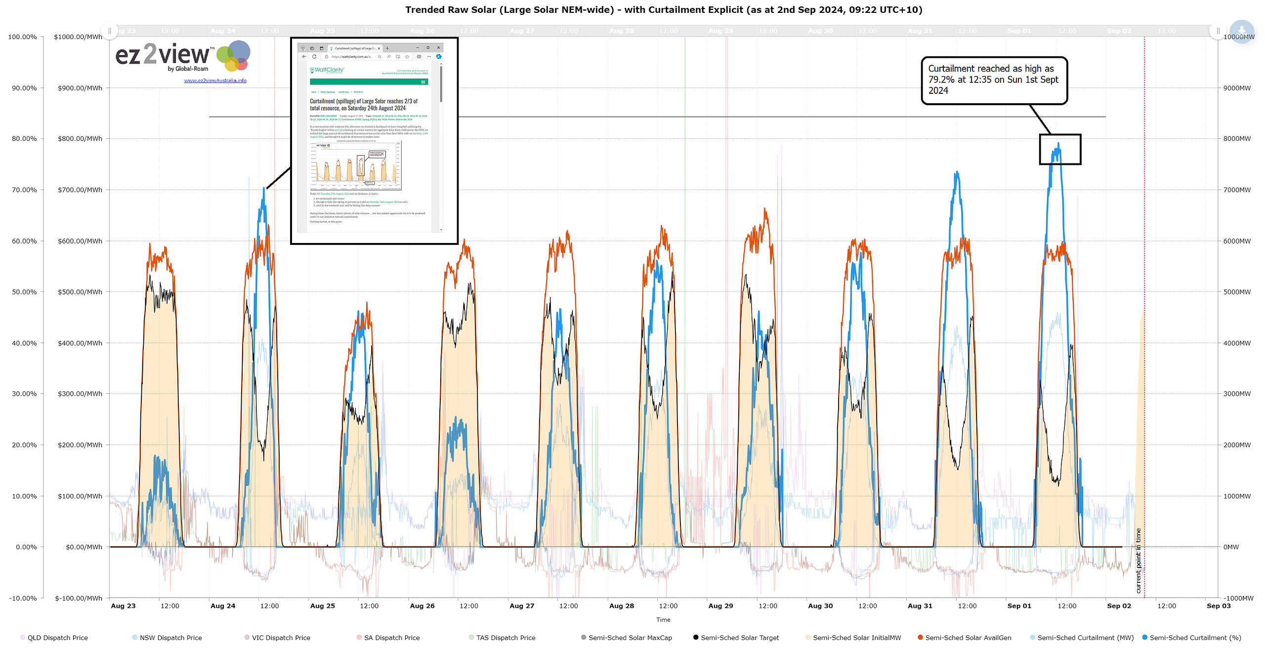
It’s barely spring in Australia and already we’re reaching the point where there’s too much solar. There’s such an excess of useless energy, prices are negative, meaning the hapless generators have to pay people to take the poison power away. And on Sunday, at a time when investors ought be making their peak profit for the day, they were rushing to turn 80% of their panels off.
It’s just another day of profligate waste in Renewable World
It’s barely spring in Australia and already we’re reaching the point where there’s too much solar. There’s such an excess of useless energy, prices are negative, meaning the hapless generators have to pay people to take the poison power away. And on Sunday, at a time when investors ought be making their peak profit for the day, they were rushing to turn 80% of their panels off.
Feel the pain — the stunted curve of the solar plants (below) is supposed to be the same shape as the rooftop PV.
In reality, this is how we make the parabolic curve of orbital solar physics fit a rectangular box — by building five times as much as we need and wasting most of it.
Bear in mind, this is just the start of a the lumpy road to nowhere. Even though we already have more solar panels than we can use, we’re supposed to be installing 22,000 more panels every day in Australia to reach our mystical NetZero target.
And at the moment, there’s a bite out of the daily peak, every day.
Call it “spillage”
We’ve reached this surreal point because there is more wind power than usual and it’s spring. The weather is mild, so householders don’t need as much electricity — thus the minimum demand on the grid is falling dangerously low. That’s a problem because the giant coal plants and other reliable generators need to keep running, to supply the frequency stabilization and so they can ramp up to fill the gaps.
Angela Macdonald-Smith, Australian Financial Review
[Josh Stabler, managing director at adviser Energy Edge] …said the available wind and solar resource almost exceeded total demand, but noted that renewable “spillage” – where renewable output is not made use of – was also at a record high.
“Spillage and abundance will be continuous features of the electricity market into the future and will become more common, especially during spring,” Mr Stabler said.
It’s mayhem on the market:
The 24-hour average wholesale price was negative for Victoria, South Australia and Tasmania, according to National Electricity Market data, with NSW only just in positive territory at $16.81 a megawatt-hour for the 24 hours to 3am on Monday. That compares with the four-week average price in NSW of $206.23/MWh.
So wholesale electricity prices are six times higher than they used to be, and we have an overdesigned grid with twice as much infrastructure as we need and most of the time, a lot of the capital assets are sitting around doing nothing.
And people think if we just do more it will “be cheaper”.
This essay starts with a thank-you. Willis Eschenbach has very often been a source of insight or inspiration here at WUWT. Back on 23 February 2024, Willis posted “A Curious Paleo Puzzle,” in which he drew attention to the work of James Rae, et al., (2021) Atmospheric CO2 over the Past 66 Million Years from Marine Archives.” Rae, et al., had compiled benthic d11B and alkenone proxies to produce 66-million-year proxy record of Paleocene to Holocene atmospheric CO2 (ppm). Willis’ introduction set the present study in motion. So — thank-you, Willis.
Multiply not the entities — William of Ockham. paraphrased
This essay starts with a thank-you. Willis Eschenbach has very often been a source of insight or inspiration here at WUWT. Back on 23 February 2024, Willis posted “A Curious Paleo Puzzle,” in which he drew attention to the work of James Rae, et al., (2021) Atmospheric CO2 over the Past 66 Million Years from Marine Archives.” Rae, et al., had compiled benthic d11B and alkenone proxies to produce 66-million-year proxy record of Paleocene to Holocene atmospheric CO2 (ppm). Willis’ introduction set the present study in motion. So — thank-you, Willis.
Rae, et al., (2021) also included a 66-million-year record of d18O proxy global average sea surface temperature (SST), which Jim Hansen and colleagues had published in 2013. The usual CO2 –> T interpretation was advanced in both papers.
The solubility of CO2 is temperature-dependent. The existence of both a paleo-SST record and a paleo-CO2 record brought to mind the possibly that the rise and fall of SST was natural variation and atmospheric CO2 just followed — the Null Hypothesis.
The Null Hypothesis
The idea is that some independent natural process drove SST. The partial pressure of atmospheric CO2, P(CO2), followed SST-driven solubility. The Null Hypothesis proposes a minimalist explanation for Cenozoic SST and P(CO2). It requires no additional entity; namely the radiative forcing of CO2. A preliminary analysis looked favorable.
The idea is worked out in Cenozoic Carbon Dioxide: the 66 Ma Solution, just published and open access in MDPI Geosciences. The state of the field requires attention to the basics of the typical criticism. Two anonymous reviewers asked for extensive revisions and clarifications. The highly qualified academic editors evaluated the revised manuscript. Submission-to-acceptance took just over a month. The whole process was completely professional. MDPI Geosciences was the second submission journal. The first submission journal held the manuscript for 3.5 months, but could not find a manuscript editor. So, that submission was stillborn.
This post sketches the results; details in the paper.
SST, CO2, and Henry’s Law
Flood Basalt Volcanism: The first step was to find whether the oceans can warm without recourse to CO2 forcing. Meet the North Atlantic Igneous Province (NAIP). The NAIP, Figure 1, contains the crustal remains of the flood basalts that erupted 56 to 52 million years before the present (MYr BP), when Greenland split off from the Eurasian land mass.
The eruptions of the NAIP produced about 6.6 million km3 of basaltic magma over a period of 3-4 million years. Typically, the main phase of flood basaltic eruptions occurred over about half the time of the full duration.
Liquid basaltic magma emerges at about 1620 K and crystallizes at 1470 K. Taking into account the heat capacity and the heat of fusion of basalt, each 1 million km3 of magma releases enough heat to warm the entire 1.338 billion km3 of the global ocean by about 0.97 C. If the thermal plume rises to occupy just the top 1 km of the world ocean, the temperature change is about 3.6 C. These numbers assume the ocean captures all the released heat, which may not be the case.
Nevertheless, the thermal impact of the 6.6 million km3 of NAIP basaltic magma alone can account for the entire increase in SST entering the post-Cretaceous Paleocene-Eocene Thermal Maximum (PETM) (discussed below). Although the NAIP eruption was accompanied by large emissions of CO2 and other gases, there is no need to invoke CO2 forcing to account for the increased SST of the PETM.
The Miocene Climate Optimum is associated with the Columbia River flood volcanism. Evidence of flood basalt volcanism occurs throughout the Phanerozoic. Correlation of climate and submarine flood basalt magmatism across deep time is outside the scope of the paper, but would seem to be a fruitful area of research.
Henry’s Law: The next order of business was to derive the relation between SST and the atmospheric partial pressure of CO2, P(CO2), across the 66 million years of the Cenozoic. Figure 2 illustrates Henry’s Law, which describes the partition of CO2, as a soluble gas, between the gas phase and the solution phase.
Typically, most dissolved CO2 is the neutral molecule. However, a small fraction of the dissolved CO2 reacts with water to produce carbonic acid (H2CO3). At the alkaline pH of the upper ocean, H2CO3 is converted into bicarbonate (HCO3−) and carbonate (CO32−). Removal of H2CO3 into carbonate means additional CO2 converts into carbonic acid (Le Chatelier).
Current oceanic ratios are: CO2, 0.5%; HCO3−, 87.4%, and; CO32−, 12.1%. In Figure 2, right, the thin aqua vertical bar shows the anticipated impact of so-called “ocean acidification” from doubled CO2: slightly less carbonate, slightly more bicarbonate, and a hair more neutral CO2. The change is pH 8.1 to pH 7.9. The surface waters remain alkaline. They will not have been acidificationized.
Figure 2: Left, Henry’s Law governs the equilibration of CO2 between gas and solution phases (paired vertical blue arrows across the aqua-white interface). Right, the distribution of CO2 and carbonate with pH in sea-water-like salt solution.
Gas-phase Partial Pressure = solution-phase concentration x the Henry’s Law Constant. 1
Henry’s Law constants vary with the molecule, with temperature, with the solvent, and with the presence of other solutes. Knowledge of any two Henry’s Law factors allows calculation of the third. Figure 3 shows the correspondence of the temperature-dependent Henry’s Law constants for CO2 in sea water (HS) with the trend of d18O proxy Cenozoic SSTs.
The temperature-dependent Henry’s Law constants for CO2 plus sea water closely track the d18O proxy Cenozoic SST.
Cenozoic CO2: The paper shows that Cenozoic P(CO2) can be reconstructed as:
P(CO2) = (fractional change in HS) x (total change in P(CO2)) + baseline offset 2
at each point across the Cenozoic.
The Rae, et al., (2021) proxy construct gave a mean P(CO2) ~1093 ppm at 66 MYr BP. At the end of the Cenozoic, the mean P(CO2) was 231 ppm during the Quaternary glacial/interglacial cycles. The Cenozoic P(CO2) = 1093 – 231 = 862 ppm.
The trend in Cenozoic P(CO2) can then be calculated using the value-added equation 2. Specifically:
P(CO2)i = [(dH0,i/dH0,t)x 862 ppm] +231 ppm, 3
where (dH0,i/dH0,t) is just the fractional change in the temperature-dependent Henry’s Law constant.
Figure 3: Blue line, d18O proxy estimate of Cenozoic SSTs (Hansen et al., (2013)). Red line, trend in Henry’s Law constant for equilibration of CO2 across the atmosphere/sea surface interface during the Cenozoic. The right ordinate is descending upwards
The proxy reconstruction of Cenozoic P(CO2) proxy points of (Rae, et al., (2021)) provided a baseline reference series for the P(CO2) trends calculated from Henry’s Law. Figure 4 shows the comparison.
Figure 4: (yellow points), proxy P(CO2) over the Cenozoic from (Rae, et al., 2021)); (purple line), 15% weighted Lowess smooth. (blue line), Cenozoic P(CO2) calculated using equation 3; red line, weighted Lowess smooth. Inset: expansion of the most recent 7.5 Ma.
Two proxy SSTs for the PETM are available. The PETM maximum SST reported by Bijl, et al. (2009) is 35 C, while the Hansen, et al., 2013 reported a PETM maximum of 28 C.
The Bijl SSTs (blue line) gave a much better match to the P(CO2) proxy points. The PETM SSTs of Hansen, et al., (Figure 3), yielded PETM P(CO2) levels generally too low.
The calculated P(CO2) trend goes through the proxy CO2 points across the first 36 MYr BP of the Cenozoic. After that, P(CO2) declined all across the Cenozoic. At 30 MYr BP, the proxy suddenly dips about 300 ppm below the Henry’s Law line. However, after 22 MYr BP, the calculated and proxy slopes are nearly parallel.
At about 3 MYr BP, (inset), the proxy points and the Henry’s Law trend merge once again while P(CO2) dereases precipitously through the Pleistocene.
[CO2]ocean of the Paleocene
Of further interest, at the beginning of the Cenozoic the mean proxy estimates of SST, 297 K, and of P(CO2), 1093 ppm, allow a Henry’s Law estimate of the equilibrium concentration of CO2 in the ocean 66 million years ago. This estimate is [CO2]ocean = 3.41×10⁻⁵ Molar (M).
If the [CO2]ocean had remained constant at 3.41×10⁻⁵ M up through the present, then Henry’s Law equation 4 can reveal how atmospheric P(CO2) would have evolved through the Cenozoic given the variation in SST and under the condition of constant marine CO2.
P(CO2) = Hix 3.41x10⁻⁵ M 4
where Hi is the temperature dependent Henry’s Law constant. Figure 5 shows the result.
Figure 5: (points), proxy estimate of Cenozoic P(CO2) from Rae, et al., (2021); (purple line), Lowess smooth; (blue line), evolution of Cenozoic P(CO2) driven only by SST at constant [CO2]ocean = 3.41×10⁻⁵ M; (red line), Lowess smooth. Inset: the most recent 7.5 Ma.
At the PETM maximum (52 MYr BP), the calculated line is close to the proxy smooth, but passes through the lower region of the proxy CO2 points. This means SST alone seems unable to account for the full PETM increase in P(CO2). The volcanic activity of the NAIP probably released considerable CO2.
Heading into the Eocene and Oligocene (50-35 MYr BP), the constant [CO2]ocean trend is close to the proxy points. But after 30 MYr BP, the constant CO2 line is much higher than the proxy P(CO2) smooth. This result shows that [CO2]ocean was not constant across the Cenozoic.
An interesting revelation is that if [CO2]ocean had remained constant at 3.41×10⁻⁵ M, the post-glacial Holocene atmospheric CO2 would have been about 775 ppm. This assumes the same decreasing trend in SST to its modern value. In the Null Hypothesis, cooling would have occurred because tectonic magmatism was generally low, apart from episodic excursions such as during the MCO.
Under this scenario, industrial emissions would have increased atmospheric CO2 to about 900 ppm. There would have been no conceivable rationale at all for climate alarm, or for a war against fossil fuels. The world would also have been much greener, and the more prolific agriculture would have required conversion of far less arable wildland.
In any case, the decreasing SST alone clearly cannot account for the decline in P(CO2) after 35 MYr BP.
The modern [CO2]ocean: Henry’ Law applied to the observed post-glacial mean Holocene SST (292 K) and P(CO2) (295 ppm), yields the modern [CO2]ocean = 0.998×10⁻⁵ M.
That is, the Cenozoic has seen a loss of [(3.41 – 0.998)/3.41]x100 = 71% of the equilibrating CO2 that was present in the ocean of the Paleocene.
At constant pH, Le Chatelier says the concentration of oceanic CO2 cannot decline without a loss of bicarbonate and carbonate (Figure 2).
Therefore, the 775 – 295 = 480 ppm difference, between the a modern P(CO2) at constant [CO2]ocean, and the observed P(CO2) of the pre-industrial Holocene, quantifies the known massive Cenozoic draw-down of carbonate, which is discussed in Bestland, 2020, Dutkiewicz, et al, 2018, von Strandmann, et al., 2021, and Rae, et al., 2021.
This process began around 30 MYr BP and continued right through the Pleistocene (Figure 5).
It is unlikely that the pH of the ocean has changed much. But the modern buffer capacity is greatly diminished relative to the deep past.
The falls and rises of P(CO2) across the Quaternary glacial/interglacial cycles were driven by changes in SST alone, because they occurred without any significant change in [CO2]ocean.
The 420 kYr VOSTOK ice core records the ~100 ppm range of the global average P(CO2) cycle during the last four glacial/inter-glacial periods.
Knowing the present [CO2]ocean (0.998×10⁻⁵ M), and the d18O proxy SST over the 420 kYr period (Hansen, et al., (2013)), permits a direct calculation of the glacial/interglacial P(CO2) cycle of the Quaternary.
If the proxy SSTs are correct, the Henry’s Law P(CO2) should reproduce the VOSTOK record. The direct Henry’s Law calculation is:
P(CO2) = Hix 0.998x10⁻⁵ M, 5
where Hi is the temperature-dependent Henry’s Law constant.
Figure 6a shows that the d18O proxy SSTs yielded P(CO2) cycles that are compressed relative to the point-range of the VOSTOK record (Figure 6a, red line).
This means the temperature-dependent Henry’s Law constants were not correct. Therefore, the d18O proxy SSTs are not correct.
Figure 6: a. (points), 420 kYr of P(CO2) from the VOSTOK ice core (Petit, et al., (1999); VOSTOK data). (red line), Henry’s Law P(CO2) calculated using the d18O proxy SSTs of Hansen, et al, 2013, and the mean Quaternary [CO2]ocean = 0.998×10⁻⁵ M. b. (points), VOSTOK ice core CO2; (blue line), P(CO2) calculated using equation 2; (green line), P(CO2) directly calculated using [CO2]ocean = 0.998×10⁻⁵ M, and Henry’s Law reflecting the SST adjusted to have an 11 C glacial/interglacial range.
The accepted global average glacial/interglacial d18O proxy SST range is 4-5 C. But this range is clearly too small to reproduce the VOSTOK P(CO2) record.
Testing alternatives, only an SST with an 11 C glacial/interglacial range did a good job of reproducing the VOSTOK record (Figure 6b).
Also, only 11 C cycles yielded the correct 280 ppm P(CO2) of the pre-industrial Holocene at 0 kYr BP.
In support of this result, Cuffey et al. 2015 reported an 11.3 ±1.8 C glacial/interglacial range for West Antarctica, which they described as, “two to three times the global average.“
However, it was the Cuffey West Antarctica 11 C range that reproduced the VOSTOK global P(CO2) series (Figure 6b). This implies that 11 C is a global average range of glacial/interglacial SST, rather than confined to Antarctica.
Figure 6b shows two calculated lines. The blue line was calculated under the Null Hypothesis, equation 6
P(CO2)i = [(dH0,i/dH0,t)x 116.5 ppm] +182 ppm 6
where 116.5 ppm is the VOSTOK P(CO2) range and 182.5 ppm is the VOSTOK offset minimum.
The green line used equation 7 — the direct Henry’s Law calculation, with the modern value of [CO2]ocean = 0.998×10⁻⁵ M and Henry’s Law constants reflecting SSTs with a global average 11 C glacial/interglacial range:
P(CO2)i = Hix 0.998x10⁻⁵ M, 7
where Hi is the temperature-dependent Henry’s Law constant.
The lines of the alternative calculations almost superimpose.
An aside
The Quaternary ice ages began only after about 45 million years of ocean cooling. Equivalently large Milankovitch orbital forcing must have been present in the Cretaceous and throughout the Cenozoic, but did not produce glaciations.
Possibly, glaciations appeared because the cooling ocean eventually entered a potential energy surface that includes a bifurcation of climate states. In this view, Milankovitch orbital forcing with a lower energy flux produces a glacial icehouse climate. When orbital forcing moves to a higher energy flux, an interglacial cool-house climate is produced. The energy transition causing the climate state shift can be 100 Wm–2 at northern latitudes, and the sensitivity to the flux change appears to have been brought into being by the low SST of the Quaternary. Extended ocean cooling due to long-term quiescence of submarine flood basalt magmatism may also explain snowball Earth events.
Conclusion
The behavior of P(CO2) across the 66 million years of the Cenozoic is consistent with the Null Hypothesis.
High SSTs are produced by large scale submarine flood basalt magmatic events capable of warming the entire global ocean — about 1 C for each million km3 of eruptive basaltic magma. When an extreme magmatic event warmed the global ocean, marine CO2 outgassed into the atmosphere. When flood basaltic magmatism was quiescent, the global ocean cooled and atmospheric CO2 was absorbed.
The rises and falls of P(CO2) can be understood as physical re-equilibrations across the ocean surface in response to variations in SST, and changes in the concentrations of oxides of carbon caused by volcanism or carbonate drawdown.
Although extreme volcanic events released copious CO2, radiative forcing by CO2 is not needed to explain the high SSTs of the PETM, or of the Oligocene warm period, or of the Miocene Climate Optimum.
During the Quaternary, the cycling of P(CO2) is entirely consistent with Henry’s Law re-equilibration, as SST varied over an 11 C glacial/interglacial range.
For the past 66 million years, atmospheric CO2 can be understood as a neutral spectator molecule, right up through the present.
A short commentary
What current research reveals about consensus climatology:
2. Absent climate models, there is no evidence whatever that CO2 emissions have done, are doing, will do, or can do, anything to global air temperature.
3. The surface air temperature record is climatologically useless: here, and here, and the published field calibration experiments referenced in those papers.
The post below updates the UAH record of air temperatures over land and ocean. Each month and year exposes again the growing disconnect between the real world and the Zero Carbon zealots. It is as though the anti-hydrocarbon band wagon hopes to drown out the data contradicting their justification for the Great Energy Transition. Yes, there has been warming from an El Nino buildup coincidental with North Atlantic warming, but no basis to blame it on CO2.
The post below updates the UAH record of air temperatures over land and ocean. Each month and year exposes again the growing disconnect between the real world and the Zero Carbon zealots. It is as though the anti-hydrocarbon band wagon hopes to drown out the data contradicting their justification for the Great Energy Transition. Yes, there has been warming from an El Nino buildup coincidental with North Atlantic warming, but no basis to blame it on CO2.
As an overview consider how recent rapid cooling completely overcame the warming from the last 3 El Ninos (1998, 2010 and 2016). The UAH record shows that the effects of the last one were gone as of April 2021, again in November 2021, and in February and June 2022 At year end 2022 and continuing into 2023 global temp anomaly matched or went lower than average since 1995, an ENSO neutral year. (UAH baseline is now 1991-2020). Now we have an usual El Nino warming spike of uncertain cause, unrelated to steadily rising CO2 and now moderating.
For reference I added an overlay of CO2 annual concentrations as measured at Mauna Loa. While temperatures fluctuated up and down ending flat, CO2 went up steadily by ~60 ppm, a 15% increase.
Furthermore, going back to previous warmings prior to the satellite record shows that the entire rise of 0.8C since 1947 is due to oceanic, not human activity.
The animation is an update of a previous analysis from Dr. Murry Salby. These graphs use Hadcrut4 and include the 2016 El Nino warming event. The exhibit shows since 1947 GMT warmed by 0.8 C, from 13.9 to 14.7, as estimated by Hadcrut4. This resulted from three natural warming events involving ocean cycles. The most recent rise 2013-16 lifted temperatures by 0.2C. Previously the 1997-98 El Nino produced a plateau increase of 0.4C. Before that, a rise from 1977-81 added 0.2C to start the warming since 1947.
Importantly, the theory of human-caused global warming asserts that increasing CO2 in the atmosphere changes the baseline and causes systemic warming in our climate. On the contrary, all of the warming since 1947 was episodic, coming from three brief events associated with oceanic cycles. And now in 2024 we have seen an amazing episode with a temperature spike driven by ocean air warming in all regions, along with rising NH land temperatures, now receding from its peak.
Chris Schoeneveld has produced a similar graph to the animation above, with a temperature series combining HadCRUT4 and UAH6. H/T WUWT
August 2024 Most Regions Cooler Offset by SH Land Spike
With apologies to Paul Revere, this post is on the lookout for cooler weather with an eye on both the Land and the Sea. While you heard a lot about 2020-21 temperatures matching 2016 as the highest ever, that spin ignores how fast the cooling set in. The UAH data analyzed below shows that warming from the last El Nino had fully dissipated with chilly temperatures in all regions. After a warming blip in 2022, land and ocean temps dropped again with 2023 starting below the mean since 1995. Spring and Summer 2023 saw a series of warmings, continuing into October, followed by cooling.
UAH has updated their tlt (temperatures in lower troposphere) dataset for August 2024. Posts on their reading of ocean air temps this month are ahead of the update from HadSST4. I posted last month on SSTs using HadSST4 Oceans Warming Uptick July 2024.These posts have a separate graph of land air temps because the comparisons and contrasts are interesting as we contemplate possible cooling in coming months and years.
Sometimes air temps over land diverge from ocean air changes. Last February 2024, both ocean and land air temps went higher driven by SH, while NH and the Tropics cooled slightly, resulting in Global anomaly matching October 2023 peak. Then in March Ocean anomalies cooled while Land anomalies rose everywhere. After a mixed pattern in April, the May anomalies were back down led by a large drop in NH land, and a smaller ocean decline in all regions. In June all Ocean regions dropped down, as well as dips in SH and Tropical land temps. In July all Oceans were unchanged except for Tropical warming, while all land regions rose slightly. Now in August we see a warming leap in SH land, slight Land cooling elsewhere, a dip in Tropical Ocean temp and slightly elswhere. End result is a small upward bump.
Note: UAH has shifted their baseline from 1981-2010 to 1991-2020 beginning with January 2021. In the charts below, the trends and fluctuations remain the same but the anomaly values changed with the baseline reference shift.
Presently sea surface temperatures (SST) are the best available indicator of heat content gained or lost from earth’s climate system. Enthalpy is the thermodynamic term for total heat content in a system, and humidity differences in air parcels affect enthalpy. Measuring water temperature directly avoids distorted impressions from air measurements. In addition, ocean covers 71% of the planet surface and thus dominates surface temperature estimates. Eventually we will likely have reliable means of recording water temperatures at depth.
Recently, Dr. Ole Humlum reported from his research that air temperatures lag 2-3 months behind changes in SST. Thus cooling oceans portend cooling land air temperatures to follow. He also observed that changes in CO2 atmospheric concentrations lag behind SST by 11-12 months. This latter point is addressed in a previous post Who to Blame for Rising CO2?
After a change in priorities, updates are now exclusive to HadSST4. For comparison we can also look at lower troposphere temperatures (TLT) from UAHv6 which are now posted for August. The temperature record is derived from microwave sounding units (MSU) on board satellites like the one pictured above. Recently there was a change in UAH processing of satellite drift corrections, including dropping one platform which can no longer be corrected. The graphs below are taken from the revised and current dataset.
The UAH dataset includes temperature results for air above the oceans, and thus should be most comparable to the SSTs. There is the additional feature that ocean air temps avoid Urban Heat Islands (UHI). The graph below shows monthly anomalies for ocean air temps since January 2015.
Note 2020 was warmed mainly by a spike in February in all regions, and secondarily by an October spike in NH alone. In 2021, SH and the Tropics both pulled the Global anomaly down to a new low in April. Then SH and Tropics upward spikes, along with NH warming brought Global temps to a peak in October. That warmth was gone as November 2021 ocean temps plummeted everywhere. After an upward bump 01/2022 temps reversed and plunged downward in June. After an upward spike in July, ocean air everywhere cooled in August and also in September.
After sharp cooling everywhere in January 2023, all regions were into negative territory. Note the Tropics matched the lowest value, but since have spiked sharply upward +1.7C, with the largest increases in April to July, and continuing through adding to a new high of 1.3C January to March 2024. In April and May that started dropping in all regions. June showed a sharp decline everywhere, led by the Tropics down 0.5C. The Global anomaly fell to nearly match the September 2023 value. In July, the Tropics rose slightly while SH, NH and the Global Anomaly were unchanged. Now in August a drop in the Tropics, with little NH cooling and Global Ocean anomaly slightly lower.
Land Air Temperatures Tracking in Seesaw Pattern
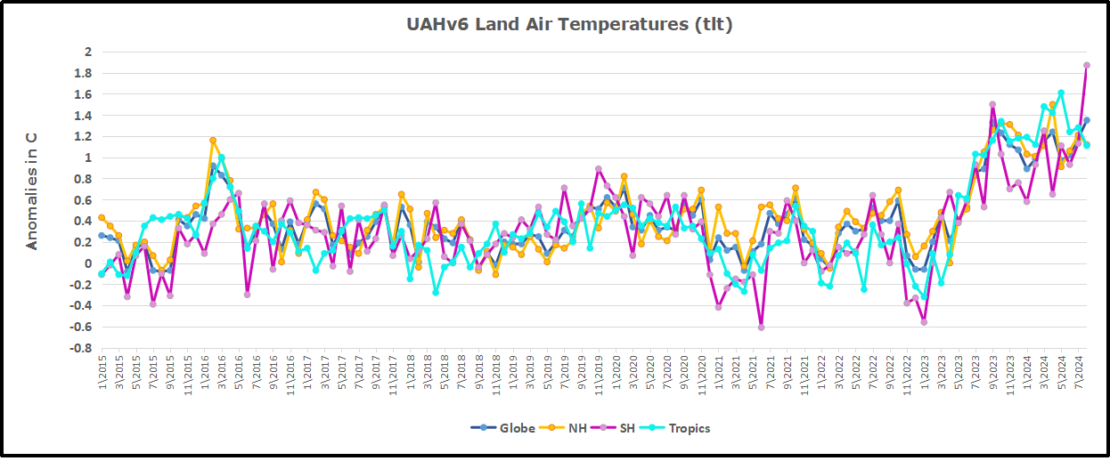
We sometimes overlook that in climate temperature records, while the oceans are measured directly with SSTs, land temps are measured only indirectly. The land temperature records at surface stations sample air temps at 2 meters above ground. UAH gives tlt anomalies for air over land separately from ocean air temps. The graph updated for August is below.
Here we have fresh evidence of the greater volatility of the Land temperatures, along with extraordinary departures by SH land. Land temps are dominated by NH with a 2021 spike in January, then dropping before rising in the summer to peak in October 2021. As with the ocean air temps, all that was erased in November with a sharp cooling everywhere. After a summer 2022 NH spike, land temps dropped everywhere, and in January, further cooling in SH and Tropics offset by an uptick in NH.
Remarkably, in 2023, SH land air anomaly shot up 2.1C, from -0.6C in January to +1.5 in September, then dropped sharply to 0.6 in January 2024, matching the SH peak in 2016. Then in February and March SH anomaly jumped up nearly 0.7C, and Tropics went up to a new high of 1.5C, pulling up the Global land anomaly to match 10/2023. In April SH dropped sharply back to 0.6C, Tropics cooled very slightly, but NH land jumped up to a new high of 1.5C, pulling up Global land anomaly to its new high of 1.24C.
In May that NH spike started to reverse. Despite warming in Tropics and SH, the much larger NH land mass pulled the Global land anomaly back down to the February value. In June, sharp drops in SH and Tropics land temps overcame an upward bump in NH, pulling Global land anomaly down to match last December. In July, all land regions rose slightly, and now in August a record spike up to 1.87 and pulling the Global land anomaly up by 0.17°C. Despite this land warming, the Global land and ocean combined anomaly rose only 0.03°C.
The Bigger Picture UAH Global Since 1980
The chart shows monthly Global anomalies starting 01/1980 to present. The average monthly anomaly is -0.04, for this period of more than four decades. The graph shows the 1998 El Nino after which the mean resumed, and again after the smaller 2010 event. The 2016 El Nino matched 1998 peak and in addition NH after effects lasted longer, followed by the NH warming 2019-20. An upward bump in 2021 was reversed with temps having returned close to the mean as of 2/2022. March and April brought warmer Global temps, later reversed
With the sharp drops in Nov., Dec. and January 2023 temps, there was no increase over 1980. Then in 2023 the buildup to the October/November peak exceeded the sharp April peak of the El Nino 1998 event. It also surpassed the February peak in 2016. After March and April took the Global anomaly to a new peak of 1.05C. The cool down started with May dropping to 0.90C, and in June a further decline to 0.80C. Despite an uptick to 0.85 in July, it remains to be seen whether El Nino will weaken or gain strength, and it whether we are past the recent peak.
The graph reminds of another chart showing the abrupt ejection of humid air from Hunga Tonga eruption.
TLTs include mixing above the oceans and probably some influence from nearby more volatile land temps. Clearly NH and Global land temps have been dropping in a seesaw pattern, nearly 1C lower than the 2016 peak. Since the ocean has 1000 times the heat capacity as the atmosphere, that cooling is a significant driving force. TLT measures started the recent cooling later than SSTs from HadSST4, but are now showing the same pattern. Despite the three El Ninos, their warming has not persisted prior to 2023, and without them it would probably have cooled since 1995. Of course, the future has not yet been written.
Guest Post by: The Competitive Enterprise Institute, The Heartland Institute, the Energy & Environmental Legal Institute, the Committee for a Constructive Tomorrow, and the International Climate Science Coalition, and Truth in Energy and Climate.
Editor’s note: This summary serves as a fact check on the biggest false claims made in the media in August, 2024.
Guest Post by: The Competitive Enterprise Institute, The Heartland Institute, the Energy & Environmental Legal Institute, the Committee for a Constructive Tomorrow, and the International Climate Science Coalition, and Truth in Energy and Climate.
Editor’s note: This summary serves as a fact check on the biggest false claims made in the media in August, 2024.
As has been the case for the past year, NASA satellite data has its “average global temperature” running warmer:
Meanwhile, the average of real-time surface stations measurements as presented by Temperature.global still has the Earth in a cooling trend since January 2015.
Finally, we’ll close by noting that although the Washington Post bemoaned the US summer as “another brutally hot summer,” the average maximum temperature for the US in August 2024 was 2°F cooler than for August 1983. That’s 41 years of emission-driven warming down the drain.
Until next month, check out these and more fact checks at:
Like the Jeopardy! game show, green energy subsidies have been Congress’ answer to every energy policy question. The first OPEC oil embargo of 1973-74 catalyzed decades of energy policy, including the formation of the Department of Energy. Wind, solar, and hydropower subsidies began in earnest with the Public Utilities Regulatory Policy Act of 1978. Similarly, subsidies for corn-based ethanol were enacted as part of the National Energy Conservation Policy Act of 1978. Both were designed to reduce the country’s dependence on Middle East oil.
Like the Jeopardy! game show, green energy subsidies have been Congress’ answer to every energy policy question. The first OPEC oil embargo of 1973-74 catalyzed decades of energy policy, including the formation of the Department of Energy. Wind, solar, and hydropower subsidies began in earnest with the Public Utilities Regulatory Policy Act of 1978. Similarly, subsidies for corn-based ethanol were enacted as part of the National Energy Conservation Policy Act of 1978. Both were designed to reduce the country’s dependence on Middle East oil.
The PURPA subsidies set off a race by independent developers to construct small generating plants whose output electric utilities were required to purchase at administratively set prices. In some cases, the subsidies were independent of how much electricity the plants actually produced, creating the moniker “PURPA machines,” because their real purpose was to extract subsidies; producing electricity was secondary.
The Energy Policy Act of 1992 modified those subsidies, creating a “temporary” production tax credit for wind power and certain types of biomass generation. Congress also enacted an Investment Tax Credit, initially for solar energy, but later extended to all renewables, which could choose between the ITC and the PTC. Although the PTC was supposed to expire in 1999, it has been repeatedly extended and expanded, most recently in the Inflation Reduction Act. The PTC now includes all zero-emissions generation, including new nuclear plants. Under the IRA, the ITC has been increased, with qualifying green energy investments able to claim a credit of as much as 60% of their construction cost.
Moreover, the IRA extends the PTC and ITC until greenhouse gas emissions from electric generation fall to just 25% of their 2005 levels, after which they will be decreased gradually. According to the U.S. Energy Information Administration, the expected date for reaching that goal is 2048.
The IRA also provides subsidies for “green” hydrogen, that is, hydrogen produced from emissions-free electricity, battery storage facilities, and facilities that capture carbon and bury it underground.
Ethanol subsidies have similarly been extended and increased, with the government now subsidizing various types of biofuels and numerous states enacting clean fuel standards, which, like renewable portfolio standards, require increasing percentages of transportation fuels to be biofuels.
Congress has not been the only institution shoveling subsidies to green energy. Many states have provided their own subsidies, especially the mid-Atlantic states that are forcing ratepayers to purchase electricity from offshore wind projects at prices many times higher than the market.. States have also enacted renewable portfolio standards forcing electric utilities to increasing percentages of electricity from renewable sources that would otherwise never be built.
This subsidy smorgasbord is supposed to reduce greenhouse gas emissions by promoting new clean energy technologies. It’s also supposed to accelerate economic growth by creating new “green” industries and high-paying jobs.
There is little evidence for the former. U.S. energy-related greenhouse gas emissions have decreased by almost 20% from 2005 levels primarily because natural gas has supplanted coal as the primary fuel for generating electricity. Between 2005 and 2023, electricity generation from natural gas was six times greater than generation from wind and solar combined. In 2023 alone, electricity generated using natural gas was three times greater than wind and solar generation.
Moreover, growth in subsidized wind and solar generation has distorted wholesale electric markets, begetting the need for subsidies to ensure existing nuclear plants continue operating, lest their owners shutter them and eliminate thousands of high-paying jobs. Enacting subsidies required to offset the distortions caused by other subsidies is surely one definition of economic insanity.
As for spurring new industries and economic growth, today, the U.S. solar manufacturing industry is moribund, with almost 90% of the solar panels installed in this country now produced in China. All but one of the offshore wind projects under construction or slated to be built are owned by European companies that their respective governments control.
The economic costs of these subsidies are borne by taxpayers, who must finance the additional deficit spending; electric ratepayers who, despite claims that renewable energy resources are less costly than traditional generating resources, have seen their electric rates soar; and drivers, who pay more for gasoline and diesel fuel as refineries have closed or been modified to produce subsidized biofuels.
Those higher costs for electricity and transportation fuels raise the costs of producing and distributing almost everything else, which ripples through the entire economy, reducing economic growth and destroying jobs.
As for green energy subsidies spurring the development of new, lower-cost clean technologies, there is nothing new about wind and solar generation that receives the lion’s share of subsidies. After almost half a century, neither are cost-competitive, especially when the additional costs of addressing their inherent intermittency are included—costs that others must pay. And new technologies, such as direct air capture of carbon, will only be commercially viable if the U.S. imposes carbon taxes of several hundred dollars per ton, which few politicians will be willing to do.
The overwhelming majority of green energy subsidies reward politically powerful constituencies and businesses whose primary purpose is not to build better energy mousetraps but to build only ones that qualify for the largest subsidies.
The government could instead target subsidies solely on true research and development efforts of new clean energy technologies, such as advanced and small modular nuclear reactors.
With the country deeply in debt, wasting hundreds of billions of dollars on subsidies for green energy, as the Inflation Reduction Act calls for, is an idea whose time is long past. Green energy Jeopardy! may be a lucrative game for the lucky recipients, but eventually everyone loses.
Jonathan Lesser is a senior fellow with the National Center for Energy Analytics and the president of Continental Economics.
This article was originally published by RealClearEnergy and made available via RealClearWire.
Green energies cannot liberate EU, which remains Russian natural gas junkie.
Showing support for peace initiatives to curb the Russia-Ukraine conflict quickly gets you labelled a Putin-appeaser here in Europe.
And just imagine the reaction you might risk getting if you called on ramping up more gas imports from Russia, where the energy is cheap and plentiful?
Incredibly, that’s what many European countries have been doing lately: importing lots of gas from Russia to meet their appetite for cheap, reliable and efficient energy.
Germany’s DPA news agency reports, citing a study by think tank Bruegel: “For the first time in almost two years, the countries of the European Union imported more natural gas from Russia than from the United States in a single quarter.”
From April to June this year, the EU purchased more than 12.7 billion cubic meters of natural gas from Russia, compared to 12.3 billion from the USA, the think tank reports. Currently Norway delivers the most gas to the EU.
Though Germany no longer purchases gas from Russia, Russia has risen to second place among suppliers across the EU.
Foreign affairs expert Norbert Röttgen of Germany’s Christian Democratic Union (CDU) has called for an EU-wide ban on imports of Russian gas. “The Europeans are supporting Ukraine with billions and at the same time paying billions into Putin’s war chest – that is neither responsible, rational nor credible,” said Röttgen.
The policy contradiction illustrates just how desperate the EU is for low-cost energy, and how EU countries don’t always dance to the music they like to play.
Meanwhile other Europeans are calling for a complete ban of the Russian energy: “Importing Russian gas equals supporting the Russian war economy and its war on Ukraine,” says Ville Niinistö, a green Finnish MEP. “We must continue to push for a total ban of Russian gas to EU markets and to limit its markets elsewhere globally as much as possible,” he told Euractiv.
FDP energy policy spokesman, Michael Kruse, on the other hand, sees the Russian imports as a source of tax revenue, and is calling for “a surcharge” on the price of Russian import gas, which could be used to help finance weapons deliveries to Ukraine. In other words, German consumers should be forced to foot the war bills by paying more for energy that is already expensive.
In August, Austria made a commitment to “phase out Russian natural gas supplies by 2027”, but that commitment was “non-binding.” Europe has obviously realized that even though it is at war with Russia, the continent still has to rely on Russia to meet its energy needs.
All that green energy hasn’t done anything – except make energy and living far more expensive, and EU citizens poorer. It’s Games Without Frontiers.
Drought has hit Schleicher County hard. Lots of the stock tanks are dry. The only plants that appear to be thriving on this part of the Edwards Plateau are scrawny mesquite trees and the ever-present prickly pear cactus.
Drought has hit Schleicher County hard. Lots of the stock tanks are dry. The only plants that appear to be thriving on this part of the Edwards Plateau are scrawny mesquite trees and the ever-present prickly pear cactus. As we turned onto County Road 339, the clouds of dust from the unpaved road were so thick that I slowed down to assure there was at least 100 yards between my vehicle and the tailgate of Ray and Sandra Pfeuffer’s pickup. It was the afternoon of August 15. The dashboard in our 4Runner showed the outside temperature was 103 F. The sun was relentless. There was almost no wind. A bare handful of clouds dotted the sky.
The Pfeuffers, who raise goats and cattle on a 3,300-acre ranch about a dozen miles southeast of Christoval, led us to a remote spot in a remote county: the Carmelite Monastery of Our Lady of Grace.
Sandra wanted me to meet the nuns at the monastery because, like the Pfeuffers and many others in Schleicher County, they were dead set against a “green” hydrogen project called Tierra Alta, that has been proposed for their neighborhood by ET Fuels, an Irish corporation that’s backed by private equity firms based in Zurich and Paris. At the monastery, we were warmly greeted by Sister Mary Grace and Sister Mary Michael. Both were quick to explain why they are opposing the project. Not only would it include dozens of wind turbines that would be visible from the monastery, it would also require lots of water. Sister Mary Grace spoke first. She told me, “We are all about prayer. We are all about justice. And we are all about people.” She went on to say the project would completely change the region’s character.
Sister Mary Michael, who relied on a wheelchair, spoke softly but cut right to the chase: “We’re in a drought, and they want to take more water,” she said. “It’s a ridiculous amount of water.”
“Ridiculous” is the right word. But the water needs of the proposed “green” hydrogen-to-methanol projects are only one absurdity in a corral-full of absurdities propelled by the outrageous amount of federal money available to corporate subsidy miners under the Inflation Reduction Act. (That legislation, you may recall, became law by a single vote, cast by Kamala Harris.) And those subsidy miners are eagerly aiming to feed at the trough. However, to collect the maximum amount of federal money under the IRA for “green” hydrogen, they will have to pave dozens, or even hundreds, of square miles of ranchland from San Angelo to Fort Stockton with wind turbines and solar panels.
As I explained here on Substack last month, the subsidies for “green” hydrogen are 1,900 times larger than what’s given to nuclear. In that piece, I quoted the late Charlie Munger, who famously said, “Show me the incentives, and I’ll show you the outcome.” I wrote, “Under rules published earlier this year by the Treasury Department and Internal Revenue Service, hydrogen producers can collect $3 per kilogram of hydrogen under the production tax credit if they use electricity from low- or no-carbon sources.” As I noted, the energy content of hydrogen is about 120 megajoules (MJ) per kilogram. When converted into Btu, that works out to a subsidy of roughly $25 per million Btu. As seen above, that means that the subsidy for green hydrogen is 11 times the current market price for natural gas.
In addition, the companies that produce “green” hydrogen may — repeat, may — also be able to collect tax credits for the energy they produce from the sun and the wind. The result, as seen in the slide above, is that for a project costing $800 million, which is the estimated cost of ET Fuels’ Tierra Alta project, the developer could collect more than half of that sum courtesy of federal taxpayers. Note that I’m hedging my statement here because the rules on the tax credits are hazy. That said, it’s clear that the 45V tax credit alone for green hydrogen could provide more than a third of the project’s cost in the first year alone.
That gobsmacking level of subsidy explains why ET Fuels, NextEra Energy, and Apex Clean Energy, are trying to develop massive “green” hydrogen projects on the Edwards Plateau. ET Fuels plans to cover 30,000 acres of ranchland in Schleicher County with 300 megawatts of wind energy capacity, 300 megawatts of solar capacity, and an unspecified amount of battery storage. That capacity will fuel a bank of electrolyzers to produce enough hydrogen for a 100,000-ton-per-year “green” methanol plant. Meanwhile, NextEra and Apex are planning projects that could dwarf what ET Fuels is proposing.
Ray, Sandra, and Jake Pfeuffer on the Pfeuffer Ranch on August 15, 2024. About the drought, Ray said, “We’ve been dry three, going on four, years now.”
When I asked the Pfeuffers why they and other leaders of The Edwards Plateau Alliance are fighting so hard to stop the hydrogen projects, they replied. “water, water, water.” Ray said, “We wouldn’t have cared if they’d built wind turbines and solar. They could’ve done whatever they wanted.” But after learning about how much water the companies wanted, Sandra said it became clear the projects “just don’t make sense.”
The ET Fuels project alone could require some 485 acre-feet of water per year or roughly 433,000 gallons per day. For perspective, that volume of water would be enough to fill more than four Olympic-size swimming pools every week. “Our aquifer can’t sustain” that much demand Ray explained. When local ranchers irrigate with center-pivot sprinkler systems, they only run their irrigation pumps for a day or two. And even that demand draws down local water wells by 15 or 20 feet until the pumping stops. The hydrogen projects will put continuous demands on the aquifer, which would be ruinous for the region’s ranchers. But that hasn’t stopped the subsidy miners.
Schleicher County, shown in red. Sign on County Road 339.
Apex Clean Energy, a subsidiary of Ares Management Corporation, a publicly traded firm based in Los Angeles that sports a market cap of $45 billion, also has big plans. In 2022, it announced it was pursuing a “green fuels hub” at the Port of Corpus Christi that would get its fuel from a massive complex of wind and solar capacity in the region near Fort Stockton. The project, known as Big Trail reportedly aims to lease 280,000 acres of land and install some 3,200 megawatts of alt-energy capacity. A map a local resident showed me indicates the company is targeting more than 700 square miles of land in Pecos County for solar and wind development. Apex, which often uses for-profit front groups to attack its opponents, has been very aggressive in its efforts to build alt-energy projects across the country. It declined to answer a list of questions that I submitted.
Florida-based NextEra Energy, the world’s biggest alt-energy producer, is planning to lease massive amounts of land in the region. The company, which has a market cap of $165 billion, is pushing a project dubbed Achilles. According to the Pfeuffers, two landmen working for NextEra told them the company aims to lease three million acres(!) of land in west Texas for alt-energy projects. Part of the land would be used for hydrogen production and the rest would be used to produce electricity for the Texas grid. The company did not respond to my emails seeking details about their project.
While these companies are leasing land in the region for hydrogen projects, it’s also clear that they face many hurdles. Local opposition, particularly in Schleicher County, is fierce. (For the record, I would not want to tangle with the nuns or Sandra Pfeuffer.) Local aquifers may be unable to produce the vast amounts of water the projects will need. According to the Pfeuffers, who attended a local water board meeting last Thursday, test wells recently drilled by ET Fuels were not overly productive.
There is plenty of market risk. Last month, Bloomberg ran a piece headlined, “Why almost nobody is buying green hydrogen.” It explained that while some 1,600 projects are on the drawing boards, “the vast majority of those projects don’t have a single customer stepping up to buy the fuel. Among the handful with some kind of fuel purchase agreement, most have vague, nonbinding arrangements that can be quietly discarded if the potential buyers back out. As a result, many of the projects…will likely never get built.” In addition, the projects are a long distance from potential markets. Apex may want to ship its fuel to maritime customers. But Fort Stockton is 456 miles from the beaches at Corpus Christi.
Finally, it’s evident that hydrogen production is, as I explained in May, “a thermodynamic obscenity.” I wrote:
Hydrogen is insanely expensive, in energy terms, to manufacture. It takes about three units of energy, in the form of electricity, to produce two units of hydrogen energy. In other words, the hydrogen economy requires scads of electricity (a high quality form of energy) to make a tiny molecule that’s hard to handle, difficult to store, and expensive to use.
The thermodynamic obscenity of making hydrogen, combined with the need to mix it with carbon dioxide (produced from somewhere else) to manufacture methanol, means that companies will encounter friction throughout the production process. As I explained to about 200 local ranchers and citizens at a free lecture I gave in Eldorado on August 15 at the Schleicher County Civic Center, the final energy output of ET Fuels’ proposed Tierra Alta project (100,000 tons of methanol per year) will be relatively small, only about 985 barrels of oil equivalent per day.
In the big picture, particularly in Texas — which produces more oil and gas than all but two or three countries — that’s a minuscule amount of energy. As seen above, the latest data from the Energy Information Administration shows that new oil wells in the Permian Basin, which is located about 150 northwest of Eldorado, are now producing about 1,300 barrels per day. And remember, that output doesn’t include the energy in the associated gas coming out of that well. And remember, the ET Fuels project will require covering some 47 square miles of ranch land with alt-energy stuff, and all of that alt-energy stuff will require using untold tons of steel, copper, concrete, wire, and untold tons of gravel for untold miles of new roads. And remember, in the Permian, a dozen or more wells are often drilled on a single multi-acre pad. Thus, while the surface footprint of the oil and gas industry is getting drastically smaller, the alt-energy sector is hoping to cover hundreds, or even thousands, of square miles of rural America with wind turbines and solar panels in its never-ending quest for ever-larger government handouts.
The punchline here is obvious: everything about the “green” hydrogen push is ridiculous. But billions in federal tax dollars are at stake. That much cash can purchase a heap of ridiculousness.
As many here know, our UAH temperature dataset is used by researchers around the world, including those who believe the more alarmist narrative of anthropogenic climate change. It has been validated with global weather balloon data in multiple peer reviewed studies.
This blog received the following comment from our alarmist friend David Appell, freelance writer:
“Roy, nobody who is serious about climate change takes you seriously. You’re a denier who has made too many mistakes. No one who knows anything is going to bother commenting here–they upset you so much that all you can think to do is block them.
You long ago left the realm of science. As they say, science advances one funeral at a time. Nobody believes your time series anyway. You did that to yourself.”
As many here know, our UAH temperature dataset is used by researchers around the world, including those who believe the more alarmist narrative of anthropogenic climate change. It has been validated with global weather balloon data in multiple peer reviewed studies.
And I’m not sure why exactly I am a “denier”; that has always mystified me. I’m even part of the supposed 97% that believes the climate system is warming partly (maybe even mostly) from our CO2 emissions. John Christy and I even published a climate sensitivity paper that assumes ALL recent warming is from CO2 emissions.
Also, I routinely allow comments here from people who disagree with me on the science. Very few people have been blocked, and those from bad behavior.
So, I think David was just having a bad day. I imagine these are difficult times for freelance writers since everyone with internet access can now be one. He’s again talking about shutting down his pro-climate alarmism, pro-COVID vaccination blog, Quark Soup. Too bad. So, for those who might want to send wishes of moral support, he can be reached at david.appell@gmail.com.



You must be logged in to post a comment.