Global warming, climate change, all these things are just a dream come true for politicians. I deal with evidence and not with frightening computer models because the seeker after truth does not put his faith in any consensus. The road to the truth is long and hard, but this is the road we must follow. People who describe the unprecedented comfort and ease of modern life as a climate disaster, in my opinion have no idea what a real problem is.
Although a 20-year period of a drier climate associated with La Nina-like conditions will dry out the biggest dead logs, so they more easily burn, changes in wildfire frequency and burnt area extent, have absolutely nothing to do with climate change.
1. There is a global fire crisis!The truth: Fires are totally driven by local conditions. Framing wildfires as a global crisis is a misleading semantic device to frame fires as part of a CO2 driven global warming narrative. For example (GRAPHIC A), the American southwest’s naturally dry climate always makes that region vulnerable to fire weather. California receives no moisture during the 4 months of summer & naturally drying vegetation. In contrast eastern USA gets most of its rains during the summer and suffers much fewer fires.
2. Wildfires have Dramatically Increased!The truth: Graphs (GRAPHIC B), only showing changes in wildfire frequency since 1950 are egregiously cherry-picking the timeline. Long term research (GRAPHIC C) shows wildfire were far more frequent before 1900. Afterwards intensive fire suppression dropped fire frequency to all time lows. However, fire suppression was allowing a dangerous accumulation of ground fuels. So, over the past 3 decades, fire suppression policies have been relaxed to allow more fires.
3. Climate Crisis Expanded Fire season to All Year! The truth: Natural fire season is caused by lightning ignitions and peaks in June thru August (GRAPHIC D blue bars). It’s human ignitions that have expanded the fire season (GRAPHIC D red bars). 85% to 95% of all fires are due to human ignitions. In the US, 13% are started by arsonists.
4. Global Warming Made Vegetation More Flammable: The truth: We all know starting a sustainable campfire requires flammable tinder and kindling (GRAPHIC E). Fire experts call tinder 1-hour fuels and kindling 10-hour and 100-hour fuels (GRAPHIC F). That means the tinder and kindling that starts wildfires only require 1 to 4 days of dry weather to become highly flammable. 1 to 4 days is weather, NOT climate. Flammable fuels that start wildfires have nothing to do with climate change which requires at least 30 years of change to detect.
5. Reporting Increased Burnt Area Fails to Mention Vegetation Type!The truth: Grass and shrub fires dominated by 1-hour and 10-hour fuels account for 70% of the burnt area since 1990. (GRAPHIC G)The extensive recent Texas panhandle fire is an example of a human ignition starting a prairie grass fire during Texas’ naturally driest month of the year. Furthermore, 1-hour fuels in grass and shrublands have increased due the increase in invasive cheat grass. Unlike most native grasses, cheat grass is an annual that dies and dries out by early spring, providing fuels for earlier fires. (GRAPHIC H)
Furthermore, in the deserts of the American southwest, limited ground fuel controls fire frequency. It once took 80 to 100 years to accumulate enough ground fuel to sustain a desert wildfire. Now cheat grass has added abundant ground fuels that have dramatically increase western USA’s desert wildfire frequency.
6. Mindlessly Blame CO2 warming for Increased Aridity! The truth: Studies of precipitation since 1998 found only 12% of the world has had any significant changes in precipitation. Only 6% has resulted in increased aridity. (GRAPHIC I) Most of that detected increased aridity in California was caused by natural La Nina-like conditions during the research’s time period.
Although a 20-year period of a drier climate associated with La Nina-like conditions will dry out the biggest dead logs, so they more easily burn, changes in wildfire frequency and burnt area extent, have absolutely nothing to do with climate change.
When she followed the link to the new Plant Hardiness map and checked our very local area, she was surprised to see that it had “warmed” here by 5°F. Here is the bit of the page she was looking at:
She was a bit perplexed by this news, as we have been having not “hot” years but cooler years recently. It took me a minute to sort through it to see that the drop down was not clear on what temperature change they were talking about. That temperature change elevated us one half a zone from zone 5b to zone 6a.
“USDA’s Plant Hardiness Zone Map is the standard by which gardeners and growers can determine which plants are most likely to thrive at a location.”
“The 2023 map is based on 30-year averages of the lowest annual winter temperatures at specific locations, is divided into 10-degree Fahrenheit zones and further divided into 5-degree Fahrenheit half-zones.”
“The 2023 map incorporates data from 13,412 weather stations compared to the 7,983 that were used for the 2012 map.”
The confusion about “Temperature Change 2012-2023” was that it is not the Global Warming type of change – average surface temperature change – but rather “30-year averages of the lowest annual winter temperatures”. Those of you who follow the odd science of averaging temperatures will see that this type of average gives a common-sense view of the most likely absolutely lowest temperature in a year expected for an area based on a 30-year climatic-period average. What hardiness zones don’t give is the lowest possible temperature.
Why do they track this particular metric?
“Plant hardiness zone designations represent what’s known as the ‘average annual extreme minimum temperature’ at a given location during a particular time period (30 years, in this instance). Put another way, the designations do not reflect the coldest it has ever been or ever will be at a specific location, but simply the average lowest winter temperature for the location over a specified time. Low temperature during the winter is a crucial factor in the survival of plants at specific locations.”
For instance, when we plant gladiolus bulbs [aka “glads”] the usual practice recommended is “In temperate zones, the corms [bulbs] of most species and hybrids should be lifted in autumn and stored over winter in a frost-free place, then replanted in spring.“ But, in our experience, when we have a mild winter, glads that we missed when lifting (digging up) in the Fall, come up in the Spring just fine. We find that aggravating, as it is a lot of work to dig them up if we could have left them in the ground. But…if one fails to lift the bulbs, and we get a hard winter, of which we have had many over the last 30 years, the majority of the glads will be frozen and lost. Now, we find that our “average lowest annual winter temperature” is -10°F to -5°F. In that range, it is possible, maybe with a lot extra care, not to dig them up. But….if we get that winter with -20°F or -10°F for a week running, we’d lose all of the glads still in the ground.
Enter the Hardiness Zone map. For our area, we are on the cusp of being able to leave glads in the ground and needing to dig them up. In the little bit of map above, we see that the green area spreading north along the Hudson River Valley from New York City. The low altitude and the warmer water of the river (comparatively warmer) keep the valley a bit warmer, as for lowest temperatures, than in the rising hills to the west and east.
Here is the whole U.S.A.:
If your area is obscured by the drop down in the middle, or you just want to see a larger version – use this link. At the USDA site, you can put in your zip code and the little drop-down report shown. You can see by the index along the right that to be totally safe from frost, temperatures below freezing, you must be in zones 10 or above.
The Arbor Day Foundation has its own versions of Hardiness Maps and interesting comparisons over the last 30 years. Why Arbor Day? “Fruit Trees for Cold Hardiness Zone 4 (Average Minimum Temperature of -30° F/-35° C) — These Apple, Cherry, Peach, Plum, Apricot, Nectarine, Pear, Asian Pear, Almond, and Walnut trees can be expected to grow and thrive in climates rated as being within USDA Cold Hardiness Zone 4. These cold hardy and resilient fruit trees are known to withstand temperatures down to -30°F / -35°C! “ [source] Also see “Orchard Frost – Critical Temperatures for Various Fruits” for common spring temperatures that can ruin orchard crops in my area.
What does all this mean? If one is going to plant expensive garden or landscaping plants, stick to the USDA Hardiness map and give yourself an extra half zone. For me, that would be sticking with my old zone 5b instead of hoping my 6a plants will survive. If I were planting a commercial orchard or nursery, I would fall back of lowest recorded temperatures for the last century or so – averages be hanged.
Personal note: My family has lived in this area for 30 years (albeit, my wife and I flitted off to the Caribbean for a decade and a bit). We have had winters with nary a flake of snow and we have had a winter that remained between -20°F and -10°F, day and night, for a week. Decimated the gardens.
As the planet has slowly come up out of the Little Ice Age, growing conditions in many places have improved with earlier frost-free dates in the Springs and later first-killing-frost dates in the Falls which add up to longer growing seasons. In some areas, this is allowing two dependable crops in the same calendar year. Hardiness Zones reflect this gentle beneficial warming.
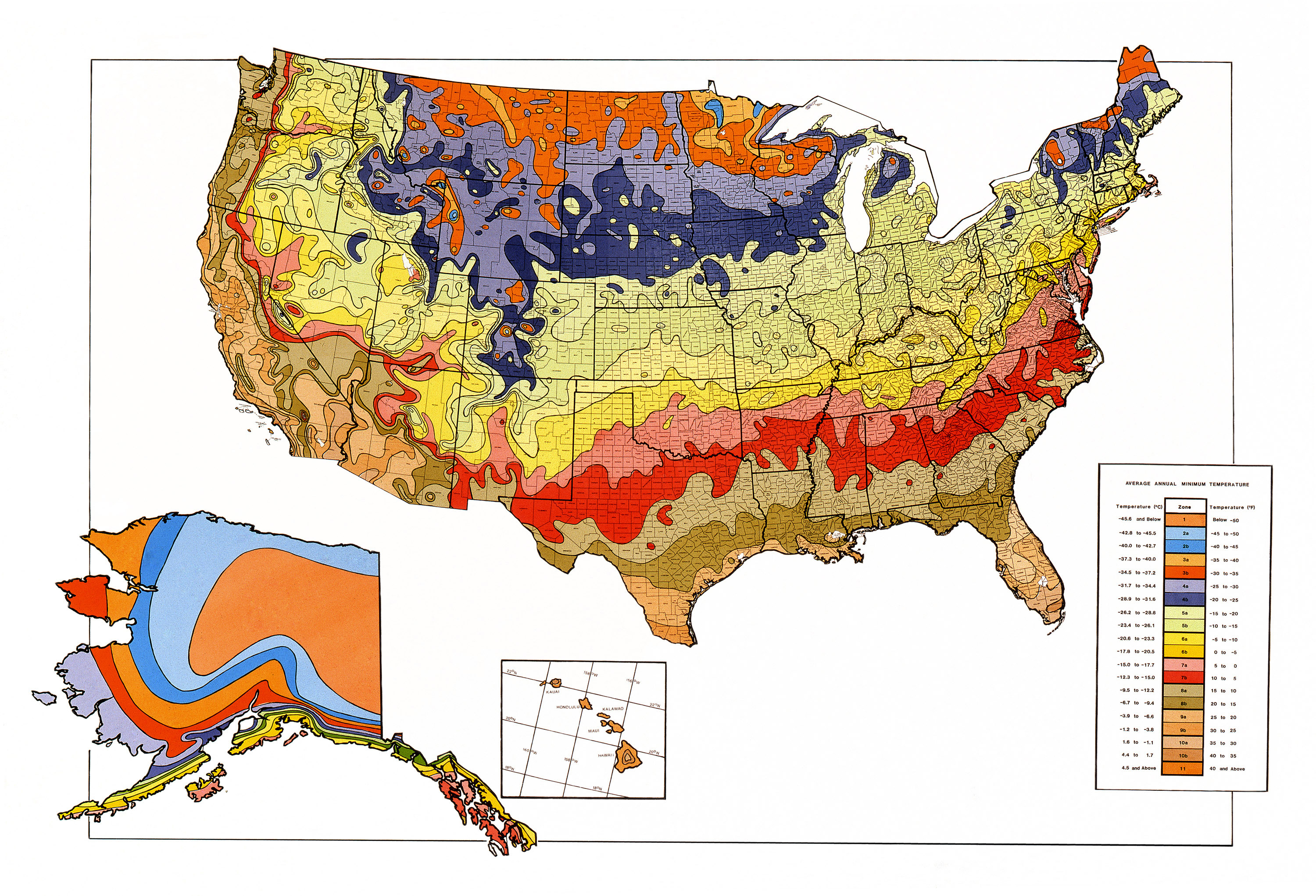
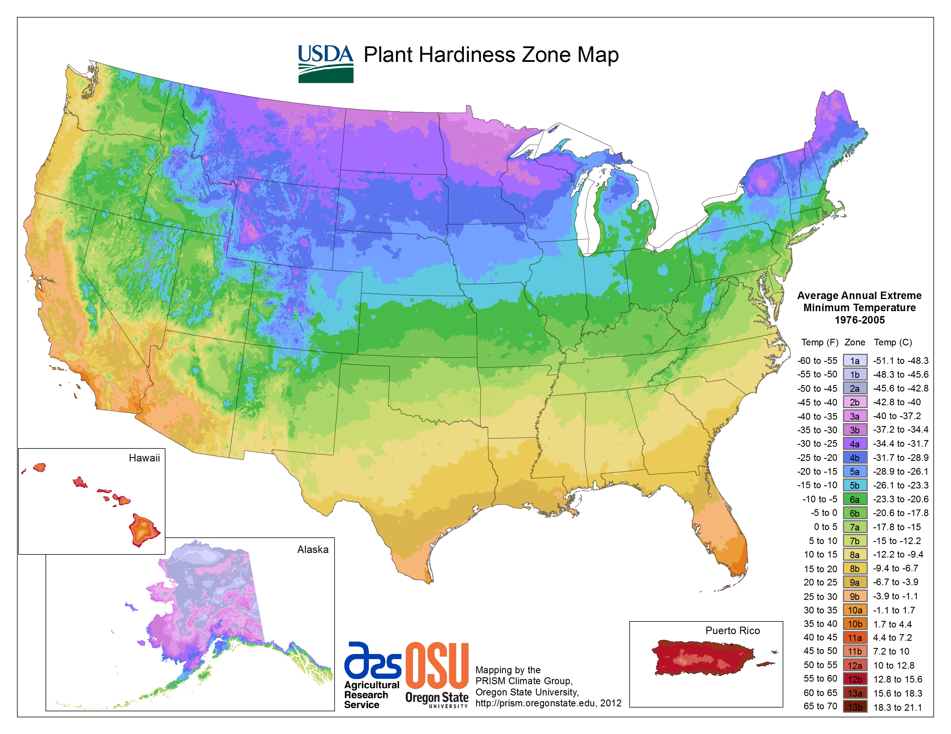
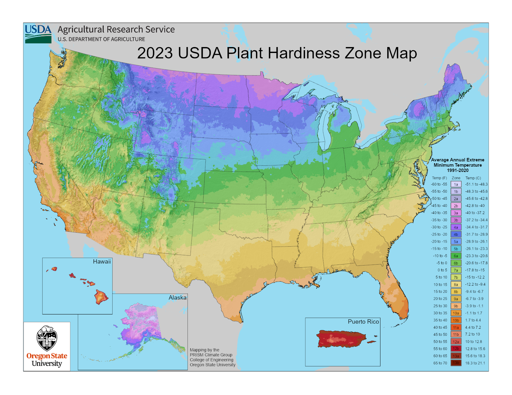
It is important to note that the USDA Hardiness Zones are now based on a great deal more data and are developed at a finer scale than previously. Here I show the 1990, 2012, and 2023 maps, side by side.
It is easy to see how coarse the map was for Alaska in the 1990 version. The differences between 2012and 2023 are very hard to see, but they are there. If you are in the United States, use this link and enter your zip code.
Bottom Lines:
1. USDA Hardiness Zones are based on “30-year averages of the lowest annual winter temperatures” – periodically, those values are re-examined and hardiness zones adjusted.
2. The changes in the Hardiness Zones represent only changes in that average.
3. The lengthening of growing seasons are a net positive for the slow gentle warming as the planet comes up out of the Little Ice Age.
# # # # #
Author’s Comment:
Not only are the U.S. Hardiness Zones changing but so are the Koopen Climate Zones – but only in modeled futures. I’ll write about that effort.
Köppen Climate Zones must be based on observations – there are no observations of the future.
The Driver Vehicle Standards Agency issued the emergency recall of 1,758 buses. A fire risk has been identified in the £800m fleet’s aircon and heating system.
The Driver Vehicle Standards Agency issued the emergency recall of 1,758 buses.A fire risk has been identified in the £800m fleet’s aircon and heating system.
Safety watchdogs have ordered the recall of almost 2,000 electric buses over fears they can catch fire if left unattended.
The Driver and Vehicle Standards Agency has warned operators who use the Alexander Dennis Enviro200 and Enviro400 single and double decker buses of the critical safety issue.
The buses are currently operational across the UK, with more than 600 in London and a further 100 in Manchester. The Daily Mail Online has the story.
All of the affected vehicles were manufactured between May 3, 2019 and February 6, 2024. They all contain batteries supplied by Chinese firm BYD.
Initial investigations suggest the fault may be in the air conditioning and heating system. The alert was issued following a scare on board one of the buses – which can cost up to £450,000 each – putting the value of the entire fleet at £800m.
At present, there is no permanent solution to prevent future fires. Instead, operators using the high-tech buses are warned to ‘switch off the Hipsacold HVAC system when the vehicle is left unattended’.
To remind drivers to isolate the power supply were they allowed to pay
Alexander Dennis told MailOnline they are working on the problem with regulators and their suppliers. They stressed the issue is not related to a string of recent fires involving ‘different vehicle types and technologies’.
In September 2021, Mayor of London Sadiq Khan announced that all new buses in London would be ‘zero emission’.
As of March 31, 2023 – most recent figures available. London had a total of 476 of the buses subject to recall in their fleet.
A further 100 of the same bus type has been supplied to Manchester as part of their move to electric buses.
Although, according to the DVSA there are almost 1,800 of the affected vehicle type on British streets.
Certain routes in the capital are now entirely electric as part of Sadiq Khan’s commitment to reduce harmful emissions in the city.
Cities such as Coventry, Birmingham, Cambridge, Leeds, Glasgow and Aberdeen also use the buses.
In London they are fitted a dedicated wheelchair space that is accessed via and electric ramp on the centre doors.
The vehicles are powered by a pair of 150kW motors from BYD on the rear drive axle.
They contain BYD Lithium-iron-phosphate batteries providing between 339kWh to 382kWh of power and are recharged at a rate of 112kW using a DC CCS2 plug.
In part 2 we discussed the IPCC hypothesis of climate change that assumes humans and our greenhouse gas emissions and land use choices are the climate change “control knob.” This hypothesis underpins their attempts to model Earth’s climate. But the model output fails to match many critical observations and in some cases the model/observation mismatches are getting worse with time.
In part 2 we discussed the IPCC hypothesis of climate change that assumes humans and our greenhouse gas emissions and land use choices are the climate change “control knob.”[1] This hypothesis underpins their attempts to model Earth’s climate. But the model output fails to match many critical observations and in some cases the model/observation mismatches are getting worse with time.[2] Since these mismatches have persisted through six major iterations of the models, it is reasonable to assume the flaw is in the assumptions, that is within the hypothesis itself, as opposed to being in the model construction. In other words, it is likely the IPCC conceptual model should be scrapped, and a new one using different assumptions constructed. In this post we examine their underlying assumption that the Sun has not varied significantly, at least from a climate perspective, over the past 150-170 years.
As well-explained by Bob Irvine,[3] there are only two things that contribute to the thermal energy content of a planet, the amount of incoming energy and the energy residence time within the system. These two things, along with the climate system heat capacity, determine the surface temperature. Arrhenius assumed and the IPCC still assumes the Sun delivers a nearly constant amount of energy to Earth over periods of a few hundred years, constant enough that it has no impact on our climate. In addition, they work with annual averages to avoid seasonal and orbital changes. In AR6, the base period is 1750 to 2019. The IPCC assumes the Sun is invariant, at least on an annual basis, over this period and volcanic activity is just slightly negative, as shown in figure 2.[4] AR6 summarizes their views as follows:
“Changes in solar and volcanic activity are assessed to have together contributed a small change of –0.02 [–0.06 to +0.02] °C since 1750 (medium confidence).”AR6 p. 962.
The change of “-0.02°C” is indistinguishable from zero. Since the IPCC assumes that solar input to Earth’s climate system does not change, temperature only varies as a function of the “energy residence time,” which they assume is controlled by human activity and greenhouse gas emissions.
As explained in part 2, greenhouse gases absorb radiation emitted by Earth’s surface and use it to warm the lower atmosphere, thus delaying its eventual escape to space. It is uncontroversial that adding more of these gases increases the delay, warming the planet’s surface.
The IPCC assumes that the radiative forcing for a doubling of CO2 from 1750 levels is 3.9[5] W/m2 or less and that the climate impact of this forcing change is roughly equivalent to a change in solar forcing of 3.9 W/m2.[6] But a 3.9 W/m2 change in greenhouse gas emissions from the atmosphere in the infrared frequencies cannot penetrate the top millimeter of the ocean. Thus, it has a different impact than a 3.9 W/m2 change in solar radiation, part of which penetrates more than 100 meters into the ocean before it is fully absorbed. Oceans cover 70% of Earth’s surface and have a low albedo (reflectivity) to sunlight, thus the oceans absorb most sunlight reaching Earth.
Figure 2. The IPCC AR6 model simulated temperature change components for the period 1750-2019. Source: AR6, p 961, figure 7.7.
Downwelling greenhouse gas radiation warms the surface of the ocean briefly, then most of it is quickly carried away by the overlying wind or as latent heat of evaporation. It has a short residence time in the ocean and in Earth’s climate system. A change in incoming solar radiation is absorbed deeper in the ocean and has a longer residence time. This increases the ocean warming effect at the point of incidence and spreads the new thermal energy over a larger volume of water. The difference in the surface warming effect can be a factor of three or more, Watt-per-Watt, relative to a change in greenhouse gas back-radiation.[7]
Evidence that Bob Irvine’s hypothesis is correct includes the change in ocean temperatures over the course of one approximately 11-year solar cycle.[8] The shallow ocean heat storage above the 22°C isotherm,[9] increases almost an order of magnitude more than the direct effect[10] of the solar cycle radiation increase. Further, this change is in phase with the solar cycle. Small changes in the Sun’s output can accumulate over time, increasing their effect on total climate system heat storage.
Wigley and Raper calculated that for a change in solar output of about 1.1 W/m2, roughly the change over one solar cycle, the direct change in Earth’s surface temperature should theoretically be in the range of 0.014°C to 0.025°C, which is undetectable.[11] However Judith Lean shows the observed surface temperature change, due to the increase in solar activity is about 0.1°C, 4 to 7 times what is expected and the increase in the upper atmosphere is 0.3°C, more than an order of magnitude more than expected from the change in radiation delivered to Earth.[12]
Lean also adds that were the Sun to become anonymously low, like during the Maunder Solar Grand Minimum (from 1645 to 1715) the expected global surface temperature cooling would still be less than a few tenths of a °C. This is only true if the cooling is linear with the change in radiation and if there are no unexpected amplifiers in the climate system, both assumptions are unlikely. We know that there are amplifiers in the climate system because the warming and cooling over the solar cycle are more than the theoretical change as Wigley and Raper have shown. The warming and cooling could be linear with the change in radiation, but there is no reason to assume this, Earth’s surface is complex and ever changing.[13]
More simply put, we know that the climate system somehow amplifies changes in insolation, but we don’t know exactly how. We know that solar output in the Maunder Solar Grand Minimum was less than now and the change from current solar output is small in percentage terms, but we have no idea what the effect on Earth’s climate of the change was, only that historical records and climate proxies suggest the effect was very large.
Known solar cycles correlate well with known climate cycles and are in phase with them.[14] Various hypotheses have been proposed to show how the Sun’s output changes over time periods of a thousand years or less. These are periods short enough to affect surface temperature from 1750, near the end of the Little Ice Age,[15] to 2019. The problem is that although a correlation between solar activity proxies[16] and climate change can be demonstrated,[17] a mechanism for the change in solar activity cannot. Attempts to explain solar variability by internal changes in the Sun only work in some cases. For example, Frank Stefani and colleagues have shown how the approximately 193-year de Vries solar cycle may be a beat period between the 22.14 Hale Solar Cycle and the 19.86-year orbit of the Sun around the solar system barycenter.[18]
Nicola Scafetta and Antonio Bianchini have shown that the orbits of the planets around the Sun correlate with solar activity proxies.[19] However, exactly how the small gravitational changes influence the solar dynamo is unclear. Thus, the hypothesis that solar activity is regulated within the Sun itself cannot completely reproduce observations, and planetary tidal forces seem too weak to accomplish the changes. These gaps in our knowledge of the mechanisms impede the acceptance that multi-centennial or multi-millennial solar changes can influence our climate. The Sun does change according to accepted solar proxies, like carbon-14 and beryllium-10 records, but the change mechanism is unclear.
The problem with the IPCC (and Arrhenius’) assumptions is that they ignore this empirical and theoretical evidence that solar output and/or solar energy input to the Earth’s climate system varies significantly over periods of a few hundred years. Their obsession with human greenhouse gases has blinded them to possible natural influences on climate change that they should be investigating. This is not to say that human greenhouse gases have no effect, it is likely that they do have some effect, but evidence suggests that natural influences, like the Modern Solar Maximum[20] and ocean oscillations,[21] play a significant role also.
There is a large body of peer-reviewed papers on the subject of solar activity as a climate change driver, yet AR6 ignores most of them. A very comprehensive review of recent research on the effect of the Sun on Earth’s climate is presented in a recent paper by Ronan Connolly and 22 colleagues.[22] In the paper they cite 396 papers on the connection between the Sun and climate, as opposed to only 68 in AR6 WG1,[23] both AR6 WG1 and the paper by Connolly, et al. were first published in 2021. This illustrates how selective the IPCC authors were in what research was considered in their report.
There is no valid reason to assume that the Sun was constant in its effect on Earth’s climate from 1750 until today. The usual reasoning is that observed changes in solar output are too small, in terms of power delivered per square meter (W/m2) relative to changes caused by increasing greenhouse gases, but as Irving explains these two sources of change are not comparable because the frequency content of the two sources are different.
Summary
The goal of this post is not to convince anyone that solar variability is responsible for all or part of modern global warming, a subject that is well covered elsewhere.[24] The point is that the IPCC reports and the CMIP models do not consider or investigate this possibility.
It is true that exactly how solar variability occurs and how it affects climate are not known, but the Sun does vary, and the variations correlate with climate changes. It is unlikely that climate changes are a direct result of the change in insolation, the solar changes are amplified by Earth’s climate system somehow.
We also do not know how much solar output has varied since 1650, the middle of the devastatingly cold Little Ice Age and the onset of the Maunder Solar Grand Minimum. There are several possible reconstructions of solar output since then. Figure 3 shows one of them constructed from an ice core beryllium-10 isotope record by Steinhilber, et al. The major climatic periods since 0AD are noted on it, and the Solar Grand Minima are identified.
Figure 3. The Steinhilber, et al. (2009) TSI reconstruction from 10berylium isotopes. The solar grand minima are identified, as well as the major climatic periods since 0AD.
The absolute values of delta-TSI (the change in total solar irradiation), in W/m2, plotted in Figure 3 are based on one of many possible modern TSI reconstructions (PMOD) and may not be accurate, but their values relative to one another are reasonable. None of the modern satellite TSI reconstructions are well supported, and the debate over which one is the best is furious and ongoing. See the discussion here for an introduction to the debate. It is best to not consider the absolute value of the Y axis in Figure 3, and consider it a TSI index, no one really knows how much TSI has changed, even over the satellite era. Further, as we’ve seen, how TSI changes relate to climate changes quantitatively is also not known. All we know is that they generally change together.
In Figure 3 we can see that colder periods, like the Little Ice Age, have some solar peaks and some warmer periods, and the Medieval Warm Period has solar lows. None of the climatic periods identified in Figure 3 were uniformly cold or warm. What we call the Little Ice Age, had some hot periods, and the Medieval Warm Period had cold periods (see the section after figure 2 here for references). Further, the correlation between solar activity and climate is not exact, nor is it uniform and synchronous over the whole planet. This is probably because of the effects of convection and atmospheric and oceanic circulation that I examine in the next post. Climate change is complicated.
The beginning and end of the climate periods identified in figure 3 are approximate, and mostly a judgement call. All the climate periods start and end at different times in different places.
However, we do know that some solar proxy reconstructions correlate well with climate proxies since 1850 (see Table 1 here),[25] and that alone is justification for additional research. Solar variability can explain anywhere from zero to almost 100% of the warming since 1850, depending upon the datasets used.[26]
This is a very brief summary of the evidence that changes in solar activity affect climate. More comprehensive discussions of possible mechanisms and the evidence for them are available.[27] Suffice it to say that this is an area of research that is too often ignored and brushed away as unimportant, especially by the IPCC. The sometimes excellent correlations in the peer-reviewed literature between solar activity and climate change alone should be enough to spur research. The fact that the IPCC has ignored these correlations is evidence of bias.
A point we will make many times in this series is that the Earth is not a uniform single thermodynamic body. Its surface is constantly changing. Treating it as a simple thermodynamic body, and one that can be characterized by a global average temperature is a huge mistake. Next, in part 4, we will discuss the potential impact of long-term changes in convection patterns.
(Lacis, Hansen, Russell, Oinas, & Jonas, 2013), (Lacis, Schmidt, Rind, & Ruedy, 2010), and (IPCC, 2021, p. 179) ↑
(McKitrick & Christy, A Test of the Tropical 200- to 300-hPa Warming Rate in Climate Models, Earth and Space Science, 2018), (McKitrick & Christy, 2020), (Lewis, 2023), (IPCC, 2021, p. 990) ↑
(Irvine, A Thought Experiment; Simplifying the Climate Riddle, 2023) and (Irvine, A comparison of the efficacy of green house gas forcing and solar forcing, 2014) ↑
(IPCC, 2021, p. 959), (Hansen, et al., 2005), and (IPCC, 2013, pp. 664-667) ↑
(Irvine, A Thought Experiment; Simplifying the Climate Riddle, 2023) and (Irvine, A comparison of the efficacy of green house gas forcing and solar forcing, 2014). Irvine provides estimates of the surface warming “efficacy” of greenhouse gas forcing versus solar forcing. ↑
An isotherm is a plane of equal temperature, in this case 22° below the ocean surface. ↑
(White, Dettinger, & Cayan, 2003). The change in radiation expected ocean temperature change is done with the Stefan-Boltzmann equation. The expected change in heat content assumes a solar cycle radiation change of about 0.1 W/m2. ↑
(Connolly et al., 2021), (Soon W. , et al., 2023), (Scafetta N. , Empirical assessment of the role of the Sun in climate change using balanced multi-proxy solar records., 2023), and (Soon, Connolly, & Connolly, 2015). ↑
(Behringer, 2010) and (May, Are fossil-fuel CO2 emissions good or bad?, 2022) ↑
(Scafetta N. , Understanding the role of the sun in climate change, 2023c) and (Scafetta N. , Empirical assessment of the role of the Sun in climate change using balanced multi-proxy solar records., 2023) ↑
(Scafetta & Bianchini, Overview of the Spectral Coherence between Planetary Resonances and Solar and Climate Oscillations, 2023b) and (Scafetta & Bianchini, The Planetary Theory of Solar Activity Variability: A Review, 2022) ↑
(Vinós & May, The Sun-Climate Effect: The Winter Gatekeeper Hypothesis (I). The search for a solar signal, 2022) and (Usoskin, Solanki, & Kovaltsov, 2007) ↑
(Vinós & May, The Winter Gatekeeper hypothesis (VII). A summary and some questions, 2022f), (Wyatt & Peters, A secularly varying hemispheric climate-signal propagation previously detected in instrumental and proxy data not detected in CMIP3 data base, 2012b), (Wyatt, Kravtsov, & Tsonis, Atlantic Multidecadal Oscillation and Northern Hemisphere’s climate variability, 2012a), and (Wyatt & Curry, 2014). ↑
(Connolly et al., 2021), (Soon, Connolly, & Connolly, Re-evaluating the role of solar variability on Northern Hemisphere temperature trends since the 19th century, 2015), (Crok & May, 2023), (Hoyt & Schatten, 1997), and (Haigh, 2011) ↑
(Soon, Connolly, & Connolly, Re-evaluating the role of solar variability on Northern Hemisphere temperature trends since the 19th century, 2015), (Connolly et al., 2021), (Soon W. , et al., 2023), (Vinós, Climate of the Past, Present and Future, A Scientific Debate, 2nd Edition, 2022), (Hoyt & Schatten, 1997), and (Haigh, 2011). ↑
A£400m scheme set up to encourage the rollout of electric buses is effectively subsidising Chinese companies to the detriment of British ones, a group of transport businesses have claimed.
British manufacturers say current scheme is slowing net zero transition.
A£400m scheme set up to encourage the rollout of electric buses is effectively subsidising Chinese companies to the detriment of British ones, a group of transport businesses have claimed.
Under the so-called Zebra initiative, local authorities and bus operators can apply for grant funding to support the purchase of zero-emission buses. The Telegraph has the story.
It is part of the ‘bus back better’ plan unveiled by the Government during the pandemic and aims to finance the purchase of 4,000 buses, accounting for around one-tenth of Britain’s total fleet.
But some companies have complained that the bidding rules exclude projects to convert existing petrol or diesel-fueled buses into electric ones – while aiding purchases of vehicles that depend on Chinese manufacturers.
Businesses such as Sheffield-based Magtec, Scarborough-based Kleanbus and Norfolk-based Equipmake argue that converting existing diesel buses – a method known as ‘repowering’ – is a greener alternative than buying new vehicles.
But they say the Government’s grant scheme currently incentivises new bus purchases instead of repowering, effectively distorting the market.
Currently, about 70pc of electric buses being purchased in the UK are Chinese-manufactured or contain Chinese-made components such as batteries, according to an analysis of official figures by Magtec.
For example, the most common bus model registered in Britain now is the Enviro bus, which is built by Shenzhen-based BYD.
But Magtec and others say operators and local authorities should also be allowed to receive grant funding for repowering. A scheme comparable to Zebra already allows for this in Scotland.
Doing so would also speed up the transition to electric buses overall, they argue, boosting the number that come into service each year.
The Met Office data goes back to 1884, but yet again the Met Office conveniently ignore the much longer CET series, which shows that February 1779 was actually warmer. This makes a nonsense of their claim that one month’s mild weather has anything to do with “climate”.
And as the CET table below shows, there have been six other Februarys above 7.0C, with none since 1998.
The UK chart also clearly shows that mild Februarys have occurred from time to time throughout the record. It is the absence of extremely cold months in the last decade or two which is largely responsible for the rise in average temperatures.
Given the fact that most of the Met Office’s temperature stations are junk, any claims that last month was a fraction of a degree warmer than, for instance 1945, cannot be treated seriously.
The BBC also talk of floods, yet although last month was much wetter than average, it was a long way from being a record, and there have been several other years with similar amounts of rainfall. It is the same story with winter rainfall as a whole.
I have already asked if the sun is setting on wind energy and now it seems we have to ask the same question about the European solar industry. A recent Politico article headline suggests (in a rather strange choice of words) that a “drowning” solar industry needs to be rescued (the body of the article says that it is “dying” rather than “drowning”). Whichever word is more apt, it seems clear that the European solar industry is in deep trouble.
So much so that we are told that the EU is urging its members to sign a joint declaration pledging to revive it. The article is quite an eye-opener, given that the mainstream media is so keen to have us believe that renewable energy is cheap and the way forward. The main points can be summarised shortly as follows:
EU solar firms are worried about an imminent collapse of their industry. In part this is said to be due to “heavily subsidised” Chinese competition. Of course, while such subsidies might be playing a role (as might the Chinese use of Uighur slave labour), no doubt the fact that Chinese energy is cheap (because they use a lot of coal) and energy within Europe is expensive (because they use a lot of renewable energy) is also highly relevant. The other issue, we are told, is a supply glut within the EU. I take that to mean that the supply of solar is significantly more than the demand for it. After years of propaganda, in other words, solar panels aren’t all that popular.
Reference is made to Meyer Burger’s recent announcement that it intends to cease module production in Germany. The text, according to pv magazine is as follows:
With a deteriorating market environment in Europe, continuing with full-scale European solar manufacturing is not sustainable for the time being. Part of the plan would unfortunately be the closure of one of Europe’s largest operational solar module production sites in Freiberg, Germany, as early as beginning of April 2024, affecting approximately 500 people.
The letter sent by the EU Commission to the energy ministers of member states talks of “the current worsening of the situation” and seeks “the signature of a declaration committing to take concrete actions to support the EU solar production.”
The Politico article suggests that the situation is so bad that this won’t placate solar manufacturers within the EU:
For months, the industry has been urging the Commission to spearhead an emergency buyout of inventories and further relax EU subsidy rules.
The EU seems to be talking about measures which are fairly obviously aimed at China, such as setting up state-led project auctions to promote the production of solar panels with “high environmental, innovation and labour standards.”
The conclusion, however, is that the situation is so dire that:
To keep the sector alive, argued Dries Acke, policy director at the SolarPower Europe lobby, the Commission “needs to become more concrete very soon” with plans to unlock EU cash.
Money. It’s always about money. Weren’t we assured that net zero would make us all better off?
Here’s another in the genre. I may make posting about these peer reviewed Science® “studies” a regular thing. There seems to be no lack of low hanging fruit.
Much of what passes for Science® these days is the construction of some focus groups given various subjective A/B tests, then followed up by detailed statistical analysis of subjective surveys of the participants. Not just “Climate Communications”. I’ve seen the same thing in other soft subjects, such as “Design Science” for years.
Here’s another in the genre. I may make posting about these peer reviewed Science® “studies” a regular thing. There seems to be no lack of low hanging fruit.
One of the more bizarre aspects of this paper is their term for vegetarians and vegans combined “veg*ans”, which feels either PC, avoiding spelling out a bad word, or religious, avoiding writing a sacred word, in its construction.
I guess their big contribution is they looked at meat eaters AND veg*ans.
Abstract
Eating meat is a prime example of cognitive conflict. Research on meat-related conflict has focused on people who eat meat (omnivores), and mostly neglected that people who avoid eating meat (vegetarians and vegans; veg*ans) can also experience conflict in the form of ambivalence. Here, we provide a conceptual model explaining how ambivalence comes to exist in omnivores and veg*ans, and how it is associated with dietary behavior. We hypothesize that ambivalence in omnivores arises when they become aware of the negative aspects of meat. Yet, even veg*ans, who predominantly hold negative attitudes towards meat, may experience ambivalence if past positive attitudes resurface. We investigated this model in a cross-sectional study (N = 1028) via the stages of change, which explain qualitative steps in people’s adoption and maintenance of new behaviors such as a veg*an diet. Our data show that meat consumption decreases linearly across the five stages of change. In line with our model, ambivalence increases from the pre-contemplation via the contemplation to the preparation stage among omnivores and decreases right after people become veg*ans (action stage) until they reach the maintenance stage. This inverted u-shaped trajectory was accompanied by a) an increase in negative evaluations of meat and b) a decrease in positive evaluations of meat from the pre-contemplation to the preparation stage. However, especially positive hedonic evaluations that render meat pleasurable partly persisted in the action stage and only dissolved in the maintenance stage. We thus argue that the observed pattern of felt ambivalence might explain why a growing number of people become open to eschewing meat and why veg*ans often eat meat and/or return to their omnivorous diets shortly after becoming veg*an.
Of course they assume all of the antiquated invalid assumptions and poor nutrition science about meat eating and production, mixed in with some truth, such as ethical considerations, and perhaps zoonotic diseases. But taking that part on is beyond the scope of this article.
Human food systems, and especially meat consumption, are responsible for some of humanity’s greatest challenges. In 2018, 69 billion chickens, 1.5 billion pigs, 656 million turkeys, 574 million sheep, 479 million goats, and 302 million cattle were slaughtered worldwide (Ritchie & Roser, 2019). To farm this number of animals, a vast amount of land and resources is necessary (Poore & Nemecek, 2018), making meat consumption a primary contributor to water and air pollution (Godfray et al., 2018, p. 361), climate change (Tilman & Clark, 2014), and biodiversity loss (Westhoek et al., 2011). Eating meat (especially processed red meat) is also linked to higher mortality rates, cardiovascular diseases, type 2 diabetes, and certain types of cancer (Afshin et al., 2019; Willett et al., 2019), and it has recently been linked to antibiotic resistance (Godfray et al., 2018, p. 361) and the spread of zoonotic diseases such as avian influenza (Espinosa et al., 2020). Thus, many people are increasingly aware of the downsides of eating meat concerning animal welfare, human health, and the environment (Godfray et al., 2018, p. 361; Joy, 2011; Siegrist et al., 2015; Willett et al., 2019).
Then they acknowledge some truth.
At the same time, many people think of meat as something positive because of its nutritional density, taste, or the cultural traditions associated with it (Leroy & Praet, 2015; Rosenfeld & Tomiyama, 2019). Indeed, meat is rich in protein, iron, and zinc. Some scholars have suggested that people learned the association between these nutrients and the taste of meat, which might have fueled people’s desire for meat’s umami taste (Griffioen-Roose et al., 2011; Morrison et al., 2012). Beyond that, meat also played a pivotal role in the evolution of human social activities, being part of many culinary rituals and traditions revolving around food up to today (Leroy & Praet, 2015). Thus, eating meat is an integral part of most societies across the world (Ruby, 2012).
People are bombarded with a lot of information both true and false. People also make observations about their own lives, health, and well-being after various choices which leads us to:
Due to the potential negative associations of meat, it is unsurprising that omnivores experience ambivalence in a variety of situations where their predominant positive attitude is opposed by negative associations (Berndsen & van der Pligt, 2004; Buttlar et al., 2023). This refers to situations where they realize meat’s downsides referring to animal welfare, health, or environmental issues, but omnivores may also experience ambivalence due to social ramifications of eating (such as discussions with veg*ans) and negative sensory experiences (such as biting into cartilage). In fact, 94.3% of omnivores in a German student sample report knowing about associations that oppose their predominant attitude (Buttlar et al., 2023); and 66.8% of omnivores in a representative German sample indicated they experience at least some conflict (Pauer et al., 2022).
Due to potential positive associations, there are also many situations in which veg*ans experience meat-related ambivalence. In contrast to omnivores, however, their ambivalence stems mostly from positive associations because they predominantly hold negative attitudes toward meat (Barr & Chapman, 2002; Buttlar et al., 2023; Buttlar & Walther, 2018). This especially occurs in situations where veg*ans consider meat’s benefits for health, acknowledge the social function of eating meat, or crave the taste of meat; thus, 70.8% of veg*an German students also report to be aware of such positive associations when being asked about their conflicts (Buttlar et al., 2023).
As felt ambivalence is discomforting, people try to resolve it (van Harreveld, van der Pligt, & de Liver, 2009). As a consequence, omnivores eat less meat and veg*ans eat more meat if they experience ambivalence (Buttlar et al., 2023). This suggests that ambivalence weakens the associations between attitude and behavior due to the presence of associations that conflict with people’s predominant attitudes (Armitage & Conner, 2000; Conner et al., 2021). It is not only the attitude-behavior link, however, that leads to these effects. In fact, both dietary groups seek information to resolve their conflict (Buttlar et al., 2023)—presumably because they anticipate that information-seeking reduces ambivalence-induced discomfort (Pauer et al., 2022). This and other processes might explain how the effects of ambivalence as a meta-cognitive conflict go beyond the effects of attitudes toward dietary behavior in omnivores and veg*ans (Buttlar et al., 2023; Pauer et al., 2023).
Now comes the Sciencey® part.
In the present research, we outline and test a conceptual model that draws on the PAST model (“past attitudes are still there”; Petty et al., 2006). The PAST model assumes that people experience ambivalence when their attitudes change. People change their attitudes if they acquire information inconsistent with their prior attitudes. Per definition, this in itself may result in ambivalence before an attitude is ultimately changed (van Harreveld et al., 2015). Regarding meat consumption, omnivores might, for instance, become aware of the negative aspects of eating meat, pertaining, for example, to animal welfare, environmental, or health issues (Berndsen & van der Pligt, 2004).
Crucially, the PAST model outlines further that ambivalence may remain even when people realize that their prior attitude is obsolete and become veg*ans. This is because past attitudes do not entirely cease after attitudes have changed. Instead, people need to tag past attitudes as wrong to repress them. Support for this notion comes from qualitative studies on meat-related conflicts. For instance, one participant in the study by Buttlar et al. (2023) stated: “Sometimes I feel a conflict towards meat when it is prepared and smells good, but I would not eat it. In these moments, I think it is wrong what I feel”. (cf. Table 1; Buttlar et al., 2023). According to the PAST model, people experience ambivalence more often when people just change their attitudes because they are more likely to fail to retrieve this tag; in comparison, people who have maintained their attitudes for a while have rejected the past attitude more often and thus more automatically retrieve the false tag (Petty et al., 2006).
2. Method
The sample consisted of 1028 participants recruited via Prolific (prolific.co). It included 514 omnivores (333 females, 171 males, 10 non-binary, Mage = 34.45, age range = 18–72) and 514 vegetarians (414 females, 86 males, 14 non-binary, Mage = 33.09, age range = 18–71). Participants completed a variety of questionnaires regarding psychological constructs related to meat consumption. This sample size was chosen to accommodate the requirements for network analyses for the development of the MAQ (see Buttlar et al., 2023).
Stages of Change. We adapted the methodology from Armitage and Arden (2007) and Klöckner (2017) to assess the stages of change. Participants were asked to select one of the following statements that most applied to them: “I currently do not eat a meat-free diet and I am not thinking about it.” (Pre-Contemplation); “I currently do not eat a meat-free diet but I think about it.” (Contemplation); “I currently intend to eat a meat-free diet but do not do so right now.” (Preparation); “I currently eat a meat-free diet but I have only begun to do so.” (Action); “I currently eat a meat-free diet and I have maintained it for a while.” (Maintenance). This way, we collected data from 222 participants in the Pre-Contemplation stage, 203 participants in the Contemplation stage, 64 participants in the Preparation stage, 20 participants in the Action stage, and 519 participants in the Maintenance stage.
Meat Ambivalence Questionnaire (MAQ). The MAQ comprises 25 items assessing ambivalence in five domains in omnivores and veg*ans (Buttlar et al., 2023). These domains entail ambivalence triggered by associations regarding animal welfare, sociability, sustainability, health, and sensory aspects of eating meat. This allowed us to assess the meat-related ambivalence rather generally via the Big MAQ (which comprises all 25 items), the Mini MAQ (which comprises five general items, i.e., one from each domain), and for all five sub-scales. Internal consistencies for the Big MAQ and its subscales were good to great for vegetarians and omnivores (all ω = 0.83; except for the socially-based subscale in vegetarians: ω = 0.78; for a detailed overview, see Buttlar et al., 2023; Study 2).
General Positive and Negative Associations. We assessed participants’ positive and negative associations towards meat with two separate items. Positive and negative evaluations are strongly related unless they are assessed by split semantic differential scales (Kaplan, 1972). These items were worded “Considering only the positive[/negative] aspects of meat consumption, while ignoring the negative[/positive] aspects, how positive[/negative] are your thoughts and/or feelings regarding meat consumption?”. Participants responded on separate 7-point scales by moving a slider from 1 (not at all positive[/negative]) to 7 (extremely positive[negative]).
Specific Positive and Negative Associations. We assessed the Motivations to Eat Meat Inventory (Hopwood et al., 2021) to measure the most common positive associations by which people explain their motivation to eat meat. These explanations include that meat consumption is necessary, normal, natural, and nice (tasty). We also assessed the Vegetarian Eating Motives Inventory (Hopwood et al., 2020) to measure the most common negative associations towards meat by which people explain why they eschew meat. These include health, environmental, and animal welfare motivations reasons.
MeatConsumption. To assess meat consumption, we used three items presented in randomized order asking for different kinds of meat (“On average, how often do you eat red meat [poultry/seafood] including side dishes and snacks? Please select one option and enter a number. (If you do not consume any red meat [poultry/seafood], select “year” and enter 0)”; (adapted from Pauer et al., 2022). Participants could then either indicate the average frequency per day, week, month, or year with which they consumed each type of meat. Independent of the type of answer, we calculated the number of servings of meat that people eat each type of meat per year. Then, we computed the sum of the total meat consumption per year across all categories.
Additional Measures. The above-mentioned variables refer to the measures needed to test our hypotheses, but the data set comprises additional variables. These variables included job status, education, political orientation, dietary centrality, dietary social support, speciesism, moral emotions (disgust, anger, guilt), moralization, information seeking, and interest in signing a petition for more plant-based food in cafeterias. It also contained a three-item measure of general felt ambivalence towards meat that did not yield good reliability in veg*ans (Buttlar et al., 2023). A detailed overview of all assessed variables can be found on the OSF (https://osf.io/5qgd4/).
What do they do with these subjective, qualitative surveys? The apply:
MATH
Table 1. Regression coefficients from SEMs predicting the MAQ scales by stages of dietary change.
MAQ scale
Stages of change 2 vs 1
Stages of change 3 vs 2
Stages of change 4 vs 3
Stages of change 5 vs 4
Polynomial Contrasts (ps < .05)
β
p
β
p
β
p
β
p
Empty Cell
Mini MAQ
.47 [.41; .53]
<.001
.05 [-.02; .11]
.153
−.10 [-.17; −.04]
.003
−.55 [-.75; −.35]
<.001
quadratic, linear, cubic
Big MAQ
.46 [.41; .52]
<.001
.05 [-.02; .11]
.152
−.077 [-.14; −.01]
.018
−.638 [-.83; −.45]
<.001
quadratic, linear
Animal
.36 [.30; .41]
<.001
.004 [-.05; .06]
.901
−.06 [-.12; .01]
.070
−.47 [-.68; −.27]
<.001
quadratic, linear
Socially
.41 [.34; .48]
<.001
.08 [.005; .15]
.034
−.08 [-.16; .002]
.054
−.519 [-.78; −.26]
<.001
quadratic, linear
Sustainability
.44 [.38; .49]
<.001
−.001 [-.06; .06]
.963
−.05 [-.12; .02]
.156
−.63 [-.70; −.56]
<.001
quadratic, linear
Health
.37 [.31; .44]
<.001
.04 [-.03; .11]
.291
−.07 [-.14; −.001]
.044
−.49 [-.69; −.29]
<.001
quadratic, linear
Sensory
.39 [.32; .46]
<.001
.10 [.02; .17]
.015
−.08 [-.16; −.002]
.041
−.60 [-.83; −.37]
<.001
quadratic, linear
Note. Beta values denote changes in the factor scores of the respective MAQ scale. Significant trends for manifest polynomial contrast analyses are reported in the last column in the order of magnitude of the estimate (i.e., stronger trends are reported first). All SEMs reached adequate model fit indices (CFI >0.95; RMSEA <0.06; SRMR <0.08; see also Appendix E for details).
The real motivation for this study, to figure out how to GET PEOPLE TO STOP EATING MEAT, becomes clear in this chart below. Where progress is denoted by moving from Omnivore to Veg*an.
Clearly revealing the authors’ clear view that positive beliefs about meat eating are inherently false.
Manfred Haferburg, power plant engineer, explains the problems of the German power grid in connection with the green energy transition at online site Achgut. The result is a very informative article. It is not primarily about blackouts due to a lack of power.
The author begins by explaining three important terms: The n-1 criterion, reactive power and instantaneous reserve.
“Let’s translate all the technical gobbledygook. The experts at the power transmission grid operators have been ‘preoccupied”‘ with the topic for a long time, but politicians have not understood it because ‘it is a very complex issue’. And then comes the kicker: the German transmission grid can no longer cope with the ‘n-1 error’ in every case. This means that if, in a tense situation, one of the large transmission lines suddenly fails due to a lightning strike, long-wave conductor vibrations in high winds and snow, sabotage or a transformer/high-voltage switch fault, ‘the electricity grid could become unbalanced’ – in other words, it could collapse in a domino effect. This could result in a partial grid failure or, in the worst case, a blackout. This time it’s not me saying this, but the team leader for system behavior in the strategic grid planning department at TransnetBW. I wrote this on this site years ago and was berated for it.”
“Here, too, an attempt at layman’s language: the large rotating generators of the power plants are ‘grid-forming’ machines; due to their large mass, they keep the frequency of 50 Hz constant in the range of seconds. For our colleagues at the Feferal Ministry of Economics and Federal Grid Agency, inertia is a physical property that ensures that power fluctuations are cushioned in a range in which the time for human intervention is too short. Wind turbines have only small masses and solar panels have no rotating parts at all, they are ‘grid-following’ with their inverters; this means that they are connected to the grid of the ‘grid-forming machines’ and do not have a stabilizing effect. Incidentally, gas-fired power plants tend to be ‘grid-following machines’. The large power plant generators have also been responsible for maintaining the voltage in the grid through reactive power control.”
At the end of the article, Haferburg comes to the conclusion that we will continue to see coal-fired power plants in operation for a very long time.
Read the full article on Achgut. (Note: Today’s modern translation tools do a pretty good job at translating the text into English)
LONGi Green Energy Technology has appealed for the West not to abandon Chinese manufacturers. But in 2021 LONGi was accused of using slave labor sourced components.
Essay by Eric Worrall
LONGi Green Energy Technology has appealed for the West not to abandon Chinese manufacturers. But in 2021 LONGi was accused of using slave labor sourced components.
World’s biggest solar company warns west not to cut out Chinese suppliers
Longi executive says costs would double, job opportunities would be lost and green targets missed
The world’s biggest solar panel manufacturer has warned that Europe and the US risk slower decarbonisation of their economies if they restrict Chinese companies from their renewable energy supply chains.
China dominates solar manufacturing, accounting for more than 80 per cent of global production following decades of deep state support, rapid domestic demand growth and intense local competition.
But western political and industry leaders have called for greater diversity in supply amid a glut of Chinese imports, as well as expressing security fears about China-made components being used in critical infrastructure.
Dennis She, vice-president of Longi Green Energy Technology, which has around 20 per cent of the global market for photovoltaic modules, told the Financial Times that western countries would “at least slow down” their transitions away from fossil fuels if they were to cut back on Chinese solar supplies. He also warned that the cost of solar panels produced without Chinese involvement in countries like the US would be “double”.
LONGi, the U.S.’s top solar-panel supplier, is exposed to possible human rights violations through its supply chain. LONGi and its subsidiaries sent at least 21% of the shipping containers that carried solar panels to U.S. ports during the second quarter of 2021, according to research firm Panjiva. Including panels from another leading manufacturer that buys material from LONGi, the company could account for as much as 30% of recent shipments.
LONGi buys polysilicon, a key ingredient in most solar panels, from at least three producers that source their raw material from Hoshine Silicon Industry Co. Ltd., according to a recent report from the Helena Kennedy Centre for International Justice at Sheffield Hallam University in the U.K.
Hoshine was hit with a U.S. import restriction in June after U.S. Customs and Border Protection, or CBP, said it found evidence that the company used forced labor at factories in China’s autonomous Xinjiang region, where Beijing is accused of suppressing Uyghurs and other Muslim minorities. LONGi has denied the allegations and the Chinese government previously has denied that it is committing human rights abuses in Xinjiang.
LONGi strenuously denies using slave labor. But how can they be sure? How can any of us be sure? Even if LONGi management are completely sincere, slave labour is allegedly a practice promoted by Chinese authorities. If allegations of slave labor are true, there would be no pressure on upstream supply chain companies to tell the truth when asked, about which of their workers get to go home at night.
So my question stands – is the alleged climate crisis serious enough that we should take even a small risk of benefiting from slave labor? Or should we close the door to Chinese products, until China admits their wrongdoing, and convincingly renounces slavery? How else can we force China to stop this abomination?


You must be logged in to post a comment.