2025 The Poisonous Tree of Climate Change

Now that Trump’s EPA is determined to reconsider its past GHG Endangerment Finding, it’s important to understand how we got here. First of all, there was the EPA’s theory basis for the finding

From Science Matters

By Ron Clutz

Now that Trump’s EPA is determined to reconsider its past GHG Endangerment Finding, it’s important to understand how we got here. First of all, there was the EPA’s theory basis for the finding:

The 3 Lines of Evidence can all be challenged by scientific studies since the 2009 ruling. The temperature records have been adjusted over time and the validity of the measurements are uncertain. The issues with climate models give many reasons to regard them as unfit for policy making. And the claim that rising CO2 caused rising Global Average Surface Temperature (GAST) is dubious, both on grounds that CO2 Infrared activity declines with higher levels, and that temperature changes precede CO2 changes on all time scales from last month’s observations to ice core proxies spanning millennia.

Thus, all the arrows claiming causal relations are flawed. The rise of atmospheric CO2 is mostly nature’s response to warming, rather than the other way around. And the earth warming since the Little Ice Age (LIA) is a welcome recovery from the coldest period in the last 10,000 years. Claims of extreme weather and rising sea levels ignore that such events are ordinary in earth history. And the health warnings are contrived in attributing them to barely noticeable warming temperatures.

Background on the Legal Precedents

This post was triggered by noticing an event some years ago. Serial valve turner Ken Ward was granted a new trial by the Washington State Court of Appeals, and he was allowed to present a “necessity defense.” This astonishingly bad ruling is reported approvingly by Kelsey Skaggs at Pacific Standard Why the Necessity Defense is Critical to the Climate Struggle. Excerpt below with my bolds.

A climate activist who was convicted after turning off an oil pipeline won the right in April to argue in a new trial that his actions were justified. The Washington State Court of Appeals ruled that Ken Ward will be permitted to explain to a jury that, while he did illegally stop the flow of tar sands oil from Canada into the United States, his action was necessary to slow catastrophic climate change.

The Skaggs article goes on to cloak energy vandalism with the history of civil disobedience against actual mistreatment and harm. Nowhere is it recognized that the brouhaha over climate change concerns future imaginary harm. How could lawyers and judges get this so wrong? It can only happen when an erroneous legal precedent can be cited to spread a poison in the public square. So, I went searching for the tree producing all of this poisonous fruit. The full text of the April 8, 2019, ruling is here.

A paper at Stanford Law School (where else?) provides a good history of the necessity defense as related to climate change activism The Climate Necessity Defense: Proof and Judicial Error in Climate Protest Cases. Excerpts in italics with my bolds.

My perusal of the text led me to the section where the merits are presented.

The typical climate necessity argument is straightforward. The ongoing effects of climate change are not only imminent, they are currently occurring; civil disobedience has been proven to contribute to the mitigation of these harms, and our political and legal systems have proven uniquely ill-equipped to deal with the climate crisis, thus creating the necessity of breaking the law to address it. As opposed to many classic political necessity defendants, such as anti-nuclear power protesters, climate activists can point to the existing (rather than speculative) nature of the targeted harm and can make a more compelling case that their protest activity (for example, blocking fossil fuel extraction) actually prevents some quantum of harm produced by global warming. pg.78

What? On what evidence is such confidence based? Later on (page 80), comes this:

Second, courts’ focus on the politics of climate change distracts from the scientific issues involved in climate necessity cases. There may well be political disagreement over the realities and effects of climate change, but there is little scientific disagreement, as the Supreme Court has noted.131

131 Massachusetts v. E.P.A., 549 U.S. 497, 499 (2007) (“The harms associated with climate change are serious and well recognized . . . [T]he relevant science and a strong consensus among qualified experts indicate that global warming threatens, inter alia, a precipitate rise in sea levels by the end of the century, severe and irreversible changes to natural ecosystems, a significant reduction in water storage in winter snowpack in mountainous regions with direct and important economic consequences, and an increase in the spread of disease and the ferocity of weather events.”).

The roots of this poisonous tree are found in citing the famous Massachusetts v. E.P.A. (2007) case decided by a 5-4 opinion of Supreme Court justices (consensus rate: 56%). But let’s see in what context lies that reference and whether it is a quotation from a source, or an issue addressed by the court. The majority opinion was written by Justice Stevens, with dissenting opinions from Chief Justice Roberts and Justice Scalia. All these documents are available at sureme.justia.com Massachusetts v. EPA, 549 U.S. 497 (2007)

From the Majority Opinion:

A well-documented rise in global temperatures has coincided with a significant increase in the concentration of carbon dioxide in the atmosphere. Respected scientists believe the two trends are related. For when carbon dioxide is released into the atmosphere, it acts like the ceiling of a greenhouse, trapping solar energy and retarding the escape of reflected heat. It is therefore a species—the most important species—of a “greenhouse gas.” Source: National Research Council:

National Research Council 2001 report titled Climate Change: An Analysis of Some Key Questions (NRC Report), which, drawing heavily on the 1995 IPCC report, concluded that “[g]reenhouse gases are accumulating in Earth’s atmosphere as a result of human activities, causing surface air temperatures and subsurface ocean temperatures to rise. Temperatures are, in fact, rising.” NRC Report 1.

Calling global warming “the most pressing environmental challenge of our time,”[Footnote 1] a group of States,[Footnote 2] local governments,[Footnote 3] and private organizations,[Footnote 4] alleged in a petition for certiorari that the Environmental Protection Agency (EPA) has abdicated its responsibility under the Clean Air Act to regulate the emissions of four greenhouse gases, including carbon dioxide. Specifically, petitioners asked us to answer two questions concerning the meaning of §202(a)(1) of the Act: whether EPA has the statutory authority to regulate greenhouse gas emissions from new motor vehicles; and if so, whether its stated reasons for refusing to do so are consistent with the statute.

EPA reasoned that climate change had its own “political history”: Congress designed the original Clean Air Act to address local air pollutants rather than a substance that “is fairly consistent in its concentration throughout the world’s atmosphere,” 68 Fed. Reg. 52927 (emphasis added); declined in 1990 to enact proposed amendments to force EPA to set carbon dioxide emission standards for motor vehicles, ibid. (citing H. R. 5966, 101st Cong., 2d Sess. (1990)); and addressed global climate change in other legislation, 68 Fed. Reg. 52927. Because of this political history, and because imposing emission limitations on greenhouse gases would have even greater economic and political repercussions than regulating tobacco, EPA was persuaded that it lacked the power to do so. Id., at 52928. In essence, EPA concluded that climate change was so important that unless Congress spoke with exacting specificity, it could not have meant the agency to address it.

Having reached that conclusion, EPA believed it followed that greenhouse gases cannot be “air pollutants” within the meaning of the Act. See ibid. (“It follows from this conclusion, that [greenhouse gases], as such, are not air pollutants under the [Clean Air Act’s] regulatory provisions …”).

Even assuming that it had authority over greenhouse gases, EPA explained in detail why it would refuse to exercise that authority. The agency began by recognizing that the concentration of greenhouse gases has dramatically increased as a result of human activities, and acknowledged the attendant increase in global surface air temperatures. Id., at 52930. EPA nevertheless gave controlling importance to the NRC Report’s statement that a causal link between the two “ ‘cannot be unequivocally established.’ ” Ibid. (quoting NRC Report 17). Given that residual uncertainty, EPA concluded that regulating greenhouse gas emissions would be unwise. 68 Fed. Reg. 52930.

The harms associated with climate change are serious and well recognized. Indeed, the NRC Report itself—which EPA regards as an “objective and independent assessment of the relevant science,” 68 Fed. Reg. 52930—identifies a number of environmental changes that have already inflicted significant harms, including “the global retreat of mountain glaciers, reduction in snow-cover extent, the earlier spring melting of rivers and lakes, [and] the accelerated rate of rise of sea levels during the 20th century relative to the past few thousand years … .” NRC Report 16.

In sum—at least according to petitioners’ uncontested affidavits—the rise in sea levels associated with global warming has already harmed and will continue to harm Massachusetts. The risk of catastrophic harm, though remote, is nevertheless real. That risk would be reduced to some extent if petitioners received the relief they seek. We therefore hold that petitioners have standing to challenge the EPA’s denial of their rulemaking petition. [Footnote 24]

In short, EPA has offered no reasoned explanation for its refusal to decide whether greenhouse gases cause or contribute to climate change. Its action was therefore “arbitrary, capricious, … or otherwise not in accordance with law.” 42 U. S. C. §7607(d)(9)(A). We need not and do not reach the question whether on remand EPA must make an endangerment finding, or whether policy concerns can inform EPA’s actions in the event that it makes such a finding. Cf. Chevron U. S. A. Inc. v. Natural Resources Defense Council, Inc., 467 U. S. 837, 843–844 (1984). We hold only that EPA must ground its reasons for action or inaction in the statute.

My Comment: Note that the citations of scientific proof were uncontested assertions by petitioners. Note also that the majority did not rule that EPA must make an endangerment finding: “We hold only that EPA must ground its reasons for action or inaction in the statute.”

From the Minority Dissenting Opinion

It is not at all clear how the Court’s “special solicitude” for Massachusetts plays out in the standing analysis, except as an implicit concession that petitioners cannot establish standing on traditional terms. But the status of Massachusetts as a State cannot compensate for petitioners’ failure to demonstrate injury in fact, causation, and redressability.

When the Court actually applies the three-part test, it focuses, as did the dissent below, see 415 F. 3d 50, 64 (CADC 2005) (opinion of Tatel, J.), on the State’s asserted loss of coastal land as the injury in fact. If petitioners rely on loss of land as the Article III injury, however, they must ground the rest of the standing analysis in that specific injury. That alleged injury must be “concrete and particularized,” Defenders of Wildlife, 504 U. S., at 560, and “distinct and palpable,” Allen, 468 U. S., at 751 (internal quotation marks omitted). Central to this concept of “particularized” injury is the requirement that a plaintiff be affected in a “personal and individual way,” Defenders of Wildlife, 504 U. S., at 560, n. 1, and seek relief that “directly and tangibly benefits him” in a manner distinct from its impact on “the public at large,” id., at 573–574. Without “particularized injury, there can be no confidence of ‘a real need to exercise the power of judicial review’ or that relief can be framed ‘no broader than required by the precise facts to which the court’s ruling would be applied.’ ” Warth v. Seldin, 422 U. S. 490, 508 (1975) (quoting Schlesinger v. Reservists Comm. to Stop the War, 418 U. S. 208, 221–222 (1974)).

The very concept of global warming seems inconsistent with this particularization requirement. Global warming is a phenomenon “harmful to humanity at large,” 415 F. 3d, at 60 (Sentelle, J., dissenting in part and concurring in judgment), and the redress petitioners seek is focused no more on them than on the public generally— it is literally to change the atmosphere around the world.

If petitioners’ particularized injury is loss of coastal land, it is also that injury that must be “actual or imminent, not conjectural or hypothetical,” Defenders of Wildlife, supra, at 560 (internal quotation marks omitted), “real and immediate,” Los Angeles v. Lyons, 461 U. S. 95, 102 (1983) (internal quotation marks omitted), and “certainly impending,” Whitmore v. Arkansas, 495 U. S. 149, 158 (1990) (internal quotation marks omitted).

As to “actual” injury, the Court observes that “global sea levels rose somewhere between 10 and 20 centimeters over the 20th century as a result of global warming” and that “[t]hese rising seas have already begun to swallow Massachusetts’ coastal land.” Ante, at 19. But none of petitioners’ declarations supports that connection. One declaration states that “a rise in sea level due to climate change is occurring on the coast of Massachusetts, in the metropolitan Boston area,” but there is no elaboration. Petitioners’ Standing Appendix in No. 03–1361, etc. (CADC), p. 196 (Stdg. App.). And the declarant goes on to identify a “significan[t]” non-global-warming cause of Boston’s rising sea level: land subsidence. Id., at 197; see also id., at 216. Thus, aside from a single conclusory statement, there is nothing in petitioners’ 43 standing declarations and accompanying exhibits to support an inference of actual loss of Massachusetts coastal land from 20th century global sea level increases. It is pure conjecture.

The Court ignores the complexities of global warming and does so by now disregarding the “particularized” injury it relied on in step one, and using the dire nature of global warming itself as a bootstrap for finding causation and redressability.

Petitioners are never able to trace their alleged injuries back through this complex web to the fractional amount of global emissions that might have been limited with EPA standards. In light of the bit-part domestic new motor vehicle greenhouse gas emissions have played in what petitioners describe as a 150-year global phenomenon, and the myriad additional factors bearing on petitioners’ alleged injury—the loss of Massachusetts coastal land—the connection is far too speculative to establish causation.

From Justice Scalia’s Dissenting Opinion

Even on the Court’s own terms, however, the same conclusion follows. As mentioned above, the Court gives EPA the option of determining that the science is too uncertain to allow it to form a “judgment” as to whether greenhouse gases endanger public welfare. Attached to this option (on what basis is unclear) is an essay requirement: “If,” the Court says, “the scientific uncertainty is so profound that it precludes EPA from making a reasoned judgment as to whether greenhouse gases contribute to global warming, EPA must say so.” Ante, at 31. But EPA has said precisely that—and at great length, based on information contained in a 2001 report by the National Research Council (NRC) entitled Climate Change Science:

“As the NRC noted in its report, concentrations of [greenhouse gases (GHGs)] are increasing in the atmosphere as a result of human activities (pp. 9–12). It also noted that ‘[a] diverse array of evidence points to a warming of global surface air temperatures’ (p. 16). The report goes on to state, however, that ‘[b]ecause of the large and still uncertain level of natural variability inherent in the climate record and the uncertainties in the time histories of the various forcing agents (and particularly aerosols), a [causal] linkage between the buildup of greenhouse gases in the atmosphere and the observed climate changes during the 20th century cannot be unequivocally established. The fact that the magnitude of the observed warming is large in comparison to natural variability as simulated in climate models is suggestive of such a linkage, but it does not constitute proof of one because the model simulations could be deficient in natural variability on the decadal to century time scale’ (p. 17).

“The NRC also observed that ‘there is considerable uncertainty in current understanding of how the climate system varies naturally and reacts to emissions of [GHGs] and aerosols’ (p. 1). As a result of that uncertainty, the NRC cautioned that ‘current estimate of the magnitude of future warming should be regarded as tentative and subject to future adjustments (either upward or downward).’ Id. It further advised that ‘[r]educing the wide range of uncertainty inherent in current model predictions of global climate change will require major advances in understanding and modeling of both (1) the factors that determine atmospheric concentrations of [GHGs] and aerosols and (2) the so-called “feedbacks” that determine the sensitivity of the climate system to a prescribed increase in [GHGs].’ Id.

“The science of climate change is extraordinarily complex and still evolving. Although there have been substantial advances in climate change science, there continue to be important uncertainties in our understanding of the factors that may affect future climate change and how it should be addressed. As the NRC explained, predicting future climate change necessarily involves a complex web of economic and physical factors including: Our ability to predict future global anthropogenic emissions of GHGs and aerosols; the fate of these emissions once they enter the atmosphere (e.g., what percentage are absorbed by vegetation or are taken up by the oceans); the impact of those emissions that remain in the atmosphere on the radiative properties of the atmosphere; changes in critically important climate feedbacks (e.g., changes in cloud cover and ocean circulation); changes in temperature characteristics (e.g., average temperatures, shifts in daytime and evening temperatures); changes in other climatic parameters (e.g., shifts in precipitation, storms); and ultimately the impact of such changes on human health and welfare (e.g., increases or decreases in agricultural productivity, human health impacts). The NRC noted, in particular, that ‘[t]he understanding of the relationships between weather/climate and human health is in its infancy and therefore the health consequences of climate change are poorly understood’ (p. 20). Substantial scientific uncertainties limit our ability to assess each of these factors and to separate out those changes resulting from natural variability from those that are directly the result of increases in anthropogenic GHGs.

“Reducing the wide range of uncertainty inherent in current model predictions will require major advances in understanding and modeling of the factors that determine atmospheric concentrations of greenhouse gases and aerosols, and the processes that determine the sensitivity of the climate system.” 68 Fed. Reg. 52930.

I simply cannot conceive of what else the Court would like EPA to say.

Conclusion

Justice Scalia laid the axe to the roots of this poisonous tree. Even the scientific source document relied on by the majority admits that claims of man- made warming are conjecture without certain evidence. This case does not prove CAGW despite it being repeatedly cited as though it did.

2025 The Legal Landscape Has Shifted For EPA

But much has changed in the legal landscape in recent years that will give opponents to Zeldin’s effort an uphill battle to fight. First is the changed make-up of the Supreme Court. When the Massachusetts v. EPA case was decided in 2007, the Court was evenly divided, consisting of four conservatives, four liberals, and Anthony Kennedy, a moderate who served as the Court’s “swing vote” in many major decisions. Kennedy was the deciding vote in that case, siding with the four liberal justices.

But conservatives hold an overwhelming 6-3 majority on today’s Supreme Court. While Chief Justice John Roberts and Associate Justice Amy Coney Barrett have occasionally sided with the Court’s three liberal justices in a handful of decisions, there is little reason to think that would happen in a reconsideration of the Massachusetts v. EPA case. That seems especially true for Justice Roberts, who wrote the dissenting opinion in the 2007 decision.

The Supreme Court’s 2024 decision in the Loper Bright Industries v. EPA case could present another major challenge for Zeldin’s opponents to overcome. In a 6-3 decision in that case, the Court reversed the longstanding Chevron Deference legal doctrine.

As I wrote at the time, [w]hen established in 1984 in a unanimous, 6-0 decision written by Justice John Paul Stevens, Chevron instructed federal courts to defer to the judgment of legal counsel for the regulatory agencies when such regulations were challenged via litigation. Since that time, agencies focused on extending their authority well outside the original intents of the governing statutes have relied on the doctrine to ensure they will not be overturned.

The existence of the Chevron deference has worked to ensure the judiciary branch of government has also been largely paralyzed to act decisively to review and overrule elements of the Biden agenda whenever the EPA, Bureau of Land Management or other agencies impose regulations that may lie outside the scope and intent of the governing statutes. In effect, this doctrine has served as a key enabler of the massive growth of what has come to be known as the US administrative state.

The question now becomes whether the current Supreme Court with its strong conservative majority will uphold its reasoning in Massachusetts v. EPA in the absence of the Chevron Deference.

The Bottom Line For Zeldin And EPA

Opponents of the expansion of EPA air regulations by the Obama and Biden presidencies have long contended that the underpinnings for those actions – Massachusetts v. EPA and the 2009 endangerment finding – were a classic legal house of cards that would ultimately come falling down when the politics and makeup of the Supreme Court shifted.

Trump and Zeldin are betting that both factors are now in favor of these major actions at EPA. Only time, and an array of major court battles to come, will tell. [Source: David Blackmon at Forbes]

Footnote:

Taking the sea level rise projected by Sea Change Boston, and through the magic of CAI (Computer-Aided Imagining), we can compare to tidal gauge observations at Boston:

EPA questions 31 major energy regulations

EPA has launched a huge regulatory reform process reconsidering 31 of its biggest energy related regulations.

From CFACT

By David Wojick

EPA has launched a huge regulatory reform process reconsidering 31 of its biggest energy related regulations.

You can see the list plus some interesting discussion here.

A lot of the war on coal is under the gun plus some really bad automotive stuff. Much of it is climate related so including the bogus CO2 Endangerment Finding is very important. If that goes away a lot of the rest might be easily killed.

Examples include coal and gas killing CO2 limits on power plants. Then there are the impossible CO2 limits on cars and trucks that are designed to force people into electric vehicles.

The really good news is the scope is way broader than just climate. It includes sweeping rules like the completely unscientific PM2.5 limits. There is also my personal favorite the rule on mercury emissions from coal fired power plants where EPA said there was no evidence but we are going to regulate it anyway.

Each of these “reconsiderations” will require a full scale rule making so there is a huge amount of work to do. Who will do this work is an interesting question given the pending job cuts plus the fact that most EPA folks love these bad rules. New hires and contracts may be coming but these multiple rule making processes will take a year or more to play through.

I think EPA has at least three different strategies for killing these bad rules. Some are easier than others and which is best for each case remains to be seen.

The most laborious strategy is a rule making based on new science. This involves a lot of research and a completely new set of technical support documents. It may well be required for reversing the Endangerment Finding but since it was done in 2009 there is plenty of newer science to draw on. That the predicted harms failed to occur is especially useful.

The somewhat easier second strategy is to simply compile the arguments against the questionable rule that were filed as comments during its rule making. In this case the new finding is that the prior finding was mistaken. It may be necessary to throw in a bit of new science but most of the research has already been done.

Mercury from coal is a likely prospect here as EPA previously admitted that they could find no physical evidence that the minor mercury emissions from coal burning were the cause of the mercury found in some lakes. The filings against this foolish rule were extensive.

The wacky PM2.5 rule is another likely candidate as PM2.5 is not even a specific substance, just a particle size. There are whole books about how ridiculous this EPA rule is.

These first two strategies use scientific arguments while the third uses a legal argument. In this case EPA simply says it did not have the legal authority to issue the rule in question. Administrator Lee Zeldin has repeatedly said that prior EPA’s have gone way beyond their mission and statutory authority. This sets the stage for rescinding prior rules as illegal.

Interestingly the recent Supreme Court rejection of the prior “Chevron doctrine” makes this legal argument stronger. That doctrine basically said the Courts must defer to the Agencies when it comes to interpreting the law. It follows that EPA rules previously deemed allowable under Chevron may no longer be allowable and EPA itself can make that determination.

Then too if the Endangerment Finding is repealed the other climate rules might all lose their legal basis. Endangerment is a necessary condition for regulatory authority under the Clean Air Act.

What is certain is that 31 big fights lie ahead making this EPA combined action a truly breathtaking event. Stay tuned to CFACT as this supreme battle unfolds.

Germany’s First Offshore Wind Farm to Be Dismantled After Just 15 Years of Operation

The Alpha Ventus offshore wind farm near German North Sea Island of Borkum is set to be dismantled after being in operation for only 15 years.

It has become too unprofitable to operate without massive subsidies.

From NoTrickZone

By P Gosselin

The Alpha Ventus offshore wind farm near German North Sea Island of Borkum is set to be dismantled after being in operation for only 15 years.

It has become too unprofitable to operate without massive subsidies.

Alpha Ventus is noted as being Germany’s first offshore wind farm. Construction works commenced in August 2007 and the first turbine was installed in July 2009. The pioneering wind farm was officially commissioned on April 27, 2010.

According to Blackout News, a decisive factor for dismantling the pioneer project is the expiration of generous subsidies made possible through Germany’s EEG renewable energies feed-in act. The subsidy meant that the Alpha Ventus wind farm got 15.4 cents per kilowatt hour after being put in operation. Now that the subsidy has run out, the wind farm operators receive only the basic tariff of 3.9 cents per kilowatt hour, thus making the farm unprofitable.

Another factor: the older Alpha Venus wind farm is being eclipsed by more modern, more efficient turbines.

Offshore wind farms have high costs

Overall, offshore wind farms are significantly more expensive to operate than onshore wind farms due increased maintenance costs, poor accessibility, harsh environments and the specialized equipment and personnel needed to conduct operational works.

Offshore wind farms are significantly more expensive to operate than onshore wind farms due to a combination of factors stemming from their challenging marine environment and remote locations.

Offshore turbines are exposed to corrosive saltwater, strong winds, large waves, and potential storms, which acts to accelerates wear and tear on components. This leads to more frequent failures and the need for more robust and expensive materials.

And when turbines break down offshore, the time required to access, diagnose, and repair them is typically much longer than for onshore turbines due to weather limitations and logistical challenges. This results in more significant losses in electricity generation and revenue.

Trial of Mann v. Steyn: Post-Trial Motions Edition

Way back in the ancient year of 2012 — before this blog had even been started — Penn State climate “scientist” Michael Mann brought a lawsuit for defamation against Mark Steyn and Rand Simberg, as well as against two websites (National Review and CEI) that had hosted the blog posts of those two individuals. Mann asserted that his reputation had been damaged by the Steyn and Simberg posts, which had compared Mann to fellow Penn Stater Jerry Sandusky. The point of comparison was that Penn State had investigated and cleared both men around the same time over allegations of misconduct — scientific misconduct in the case of Mann, sexual misconduct in the case of Sandusky.

From Manhattan Contrarian

By Francis Menton

In the succeeding years, the case went through a truly unbelievable history of procedural twists and turns, including multiple motions to dismiss and appeals. There was even an effort in 2019 to seek Supreme Court review, which the Court denied at that time; but Justice Alito issued a detailed dissent as to why he thought review should have been granted. The case finally reached trial in January 2024, by which time the two corporate entities, National Review and CEI, had been dismissed from the case, leaving only the individuals Steyn and Simberg as defendants. The trial was available for public view over the internet, and I watched substantial parts of it, leading to five blog posts over the period January 27 to February 8, 2024. Links to those five posts are here, here, here, here and here. A February 9 update to the last of those posts reported on the jury verdict that was delivered on the 8th. Readers who are at all familiar with the case will recall that the jury awarded only $1 of compensatory damages against each defendant but awarded punitive damages of $1000 against Simberg and $1 million against Steyn.

In the immediate aftermath of the verdict, the liberal press was filled with gloating that the jury had ruled in favor of their climate hero Mann. For example, my February 8, 2024, post linked to one such piece at NPR (Excerpt: “Michael Mann, among the world’s most renowned climate scientists, won a defamation case in D.C. Superior Court against two conservative writers.”)

And then the case disappeared almost completely from the news for over a year. What, you may have wondered, was happening? The answer is “post-trial motions.” In between the jury verdict and the entry of what is called the “final judgment,” which is the document that resolves and ends the case, the parties get to make various requests to the judge, either to decide issues that were not before the jury, or to modify or even vacate the jury’s verdict as being contrary to law in some respect. Sometimes, those motions are few and routine, and other times they are numerous and complex.

In just the past few days, the trial judge (Alfred Irving of the D.C. Superior Court) has at last decided most of the motions (although there is at least one substantial issue remaining to be decided, as I will discuss below.). You might ask, is 13+ months normal to decide such post-trial motions? The answer is that such a long time period is quite unusual, but not unheard of; indeed, I have seen some go even longer. Here, I thought it should not have taken nearly so long. However, in Judge Irving’s partial defense, he did put together two very thorough and detailed decisions deciding the motions, one 44 pages long, and the other 46 pages.

With Judge Irving’s decisions in hand, it is now clear that February 8, 2024, the day of the jury verdict, was the high point for Mann’s cause. Since then, the process has been slow, but all the news for Mann has been bad. The bad news actually began a couple of months ago, on January 10, 2025 when Judge Irving decided a long-pending motion of National Review to be awarded attorneys’ fees and costs for the claim against it, which had been dismissed prior to trial. The dismissal as to NR took place all the way back in 2021. D.C. law provides for recovery of attorneys’ fees and costs in certain cases for successful defendants in defamation lawsuits. Irving’s decision was that Mann must pay NR $530,820.21.

Next up, on March 4 Judge Irving issued his 44-page ruling with the all-caps title “OMNIBUS ORDER ON DEFENDANTS’ POST-TRIAL MOTIONS FOR JUDGMENT AS A MATTER OF LAW, REMITTITUR, NEW TRIAL, AND STAY OF EXECUTION OF THE JUDGMENT.” The main result in this Order is that Judge Irving dramatically reduced the punitive damages award as against Steyn by 99.5%, from $1 million to $5000.

As you can see from the title of the Order, there were actually four separate requests in the post-trial motions made by Steyn and Simberg — for “judgment as a matter of law,” for new trial, for stay of execution of judgment, and for “remittitur.” “Remittitur” means that the judge reduces the amount of damages awarded by the jury. That subject is the heart of this Order. If there was to be a major remittitur, then the other requests in the motions would obviously be of much diminished significance.

The motion for remittitur from Steyn was always likely to be granted, although the exact amount of the reduction was not known until Judge Irving ruled. The reason that remittitur was likely is that there is much case law for the propositions that (1) punitive damages cannot be too much out of proportion to actual damages, and (2) punitive damages are entirely discouraged when there are no actual damages at all. Here, the jury had awarded $1 million of punitive damages against Steyn despite finding only a nominal $1 of actual damages.

By far the most important legal precedent in this area is a 1996 case from the U.S. Supreme Court, BMW of North America v. Gore. It is quite unusual for the Supreme Court to stick its nose into civil litigation in state courts under state law; but in the Gore case, the Supreme Court found a basis in the Due Process Clause of the 14th Amendment to the U.S. Constitution to place limits on awards of punitive damages in state court actions. (Note that for these purposes the D.C. Superior Court functions as the equivalent of a state court.). In the Gore case, the Alabama Supreme Court had approved an award of $2 millions of punitive damages, although the jury in the case had found only $4,000 of actual damages. In its decision, the U.S. Supreme Court prescribed a variety of factors to determine when punitive damages are excessive under the U.S. Constitution. One of those factors is the “ratio” of the “punitive damages award . . . to the actual harm inflicted on the plaintiff.” The Supreme Court (this is Justice Stevens) stated, “When the ratio is a breathtaking 500 to 1 . . . the award must surely ‘raise a suspicious judicial eyebrow.’” The Court concluded: “{W]e are fully convinced that the grossly excessive award imposed in this case transcends the constitutional limit.” With those bits of guidance, the Supreme Court in Gore did not come up with its own figure for an allowable amount of punitive damages but rather sent the case back to the Alabama Supreme Court to figure out what to do.

In the case of Steyn, the ratio of punitive to actual damages was not 500:1, but 1 million:1. Thus you can see how the punitive damages award against Steyn was always on thin ice. Judge Irving basically recognized the Gore case as the main precedent that he had to deal with and went through its various factors in great detail to come up with the $5000 figure as the allowable amount of punitive damages. From Judge Irving’s Order, page 24:

Applying the test the Supreme Court outlined in Gore, . . . this Court finds the jury award of $1 million in punitive damages to be grossly excessive and that a remittitur of the award is appropriate. The Court discusses each of the Gore factors in turn.

And then on March 12, Judge Irving issued his 46-page Order granting a motion for sanctions that had been made by both Steyn and Simberg during the course of the trial. The full text of this Order can be found here.

Judge Irving’s Order contains a lengthy and very detailed description, including dozens of citations and quotes from the trial transcript and exhibits, of the back and forth that led to the motion for sanctions. The facts in question actually took place during the part of the trial that I had watched. You can read Judge Irving’s Order if you wish, but here is my much-condensed version from my post of January 31, 2024, which is less than one-tenth as long and cuts to the heart of the matter:

In my prior post, I devoted some space to Mann’s claim for damages, which appears to be based principally on the theory that he had lost various government research grants as a result of the allegedly defamatory blog posts of Steyn and Simberg. Last week Simberg’s lawyer Victoria Weatherford had cross-examined Mann with an interrogatory answer he had given to a question asking him to substantiate his damages by providing a list of all grants he claimed he had lost for this reason. In his answer, signed under oath, Mann had not listed any grants, and instead had objected on the ground that the whole subject was “irrelevant.” My comment was “How Mann can claim damages from lost grants after giving this answer, I have no idea.”

Well, as tends to be the case, the story proved to be much more complicated than it first appeared. On re-direct examination, Mann’s lawyer came back with a supplemental interrogatory answer that Mann had served up in 2020, which did contain a list of allegedly lost grants. That seemed like a pretty good response.

But then Ms. Weatherford got another turn on what’s called “re-cross,” and she pulled out yet another supplemental answer provided by Mann to the same interrogatory. This one was dated in 2023. In 2023 the parties were finally in the run-up to the actual trial. In the 2023 answer, there was a list of allegedly lost grants that was either the same or very similar to the list from the 2020 answer, except that the amounts of money allegedly lost as to each grant had changed in many or even most cases. (It was difficult to determine exactly everything that had changed, because they never put the two lists of grants and amounts up on the screen simultaneously for the viewers at home to compare.). Some of the changed amounts were small, but some were dramatic. In the most notable case, the “lost” grant had at first been claimed to be associated with over $9 million of lost funding; but in the amended answer the number had been changed to only about $100,000. At least as to any numbers that ever appeared on the publicly-shown screen, that $9 million amount looked to be by itself far and away the majority of the claimed lost funding.

In his responses to the questioning on re-cross, Mann justified the final amended answer as just his honest attempt to get things right. At some point he realized, he said, that if that big grant had been won, most of the $9 million would have gone to institutions other than Penn State. OK, but he had signed the previous two answers under oath. Could he really have just been “mistaken” about the $9 million? Certainly the smell of this back-and-forth was that Mann had put a fake inflated $9 million figure into his claim in an effort to intimidate the defendants with a huge number, only to change it on the eve of trial when he realized that defendants probably had the information to prove him lying in front of judge and jury.

If you should read Judge Irving’s Order, what comes through loud and clear is that the conduct of Mann and his lawyers with these damages interrogatory answers had made the judge very, very angry. The aspect of the situation that most angered the judge is that Mann’s lawyers had maneuvered to get the $9 million dollar figure into an exhibit that would go before the jury, when they knew that that figure had been withdrawn as wrong, and had been replaced by a figure a small fraction the size. Then, substantial time and resources of the defendants and the court were needed to correct the record. From Judge Irving’s Order (page 29):

Here, the Court finds, by clear and convincing evidence, that Dr. Mann, through Mr. Fontaine and Mr. Williams [his lawyers], acted in bad faith when they presented erroneous evidence and made false representations to the jury and the Court regarding damages stemming from loss of grant funding. . . . The Court does not reach this decision lightly.

So what is the remedy for this conduct? That is the piece that still remains open. At the end of this Order, Judge Irving says that the remedy will be a monetary award to the defendants of the amounts they were forced to expend to deal with Mann’s misrepresentations and to correct the record. The judge invites them to make a presentation on these matters, after which there will be a round of briefing, and then another decision. It could take additional months. How much will be awarded? My guesstimate would be in the tens of thousands, although perhaps it could even reach as high as $100,000.

So, the contours of the “final judgment” in this case are coming into view. Mann will be awarded $1001 against Simberg, and $5001 against Steyn. NR will be awarded $530,000 against Mann, and Simberg and Steyn will be awarded some additional tens of thousands from Mann. Mann will be in a very substantial financial hole, with the defendants having little incentive to compromise with him, and every incentive to go after his bank accounts and his house. Probably, Mann will be able to stave that off for some substantial period of time by means of appeals. Or perhaps Mann’s angel funders, who have paid for this case on his behalf and never had their identities disclosed, will pay off the judgment for him. Publicly, Mann will go forth continuing to claim that he “won” the case by virtue of the jury verdicts.

For me the most disappointing aspect of the whole case has been the total inability of the court system to deal with Mann’s fake science. As described in detail in my post from February 6, 2024, the defendants, particularly Simberg, put on substantial and indeed definitive evidence of the flawed “science” in Mann’s Hockey Stick reconstructions — manipulation of data, incorrect error bands, suppression of adverse verification statistics, and so forth. Mann did not even feel the need to put on any scientific evidence in response. His lawyer completely ignored this entire issue on their rebuttal case, and then did not even mention it in closing argument. And yet, the jury still made an award against the defendants. The whole issue of the fake science went completely over their heads.

The most fitting end to this case will be when whoever in the federal government pays for the University of Pennsylvania “climate science” centers pull the plug on all the funding. That can’t come soon enough.

Trump Energy Choices Saving America from Economic Disaster

Having discerned the Green New Deal as fraudulent, President Trump’s shift to maximize proven energy technologies may very well be America’s salvation from an economic disaster that climate policies were sure to deliver.

From Watts Up With That?

By Vijay Jayaraj

The forced “transition” to alternative energy – relentlessly evangelized by policymakers, environmentalists, and corporate titans – promised to save humanity from purported perils of climate change. But far from being a solution, the movement proved a perilous misadventure, fundamentally misaligned with real-world energy demands.

For decades, fossil fuels – coal, oil, and natural gas – alongside nuclear power, have met global energy needs with unmatched efficiency. Together, they account for over 84% of global energy consumption, a figure that has barely budged despite years of green rhetoric and subsidies.

Unlike wind and solar, coal and nuclear plants can churn out electricity continuously month after month, rain or shine. The amount of land and materials required for such production is but a fraction of what wind turbines and solar panels take to produce equal amounts of electrons.

Oil and natural gas fuel nearly all transportation and serve as chemical feedstock for a dizzying array of products ranging from pharmaceuticals to ubiquitous plastics – roles that so-called renewables are incapable of filling. The reliability and versatility of hydrocarbons are not luxuries but necessities. If we didn’t have fossil fuels, we would have to invent them.

The green transition’s advocates often gloss over these realities, assuming that technological breakthroughs will magically bridge the gap. But hope is not a strategy.

Germany’s Energiewende, a decades-long experiment in renewable energy, has delivered soaring electricity prices – among the highest in Europe – and required a continued use of coal to back up the intermittent production of wind and solar. In the United States, California’s aggressive push for solar and wind has led to rolling blackouts and skyrocketing utility bills. Both are examples of ideology taking precedence over sensible energy planning.

Germany and California are not anomalies but a preview of what any chaser of the green unicorn would face eventually. An imposed switch from fossil fuels is affordable only for those who can bear its inefficiencies, leaving the majority of the world with diminished living standards and shortened lives.

Moreover, energy is not a one-size-fits-all proposition. Nations are endowed with unique resources, and their energy strategies must reflect the differences. Canada, for instance, harnesses its mighty rivers to generate over 60% of its electricity from hydropower – a capacity that wind and solar can’t replicate.

France’s fleet of nuclear reactors produces over 70% of the country’s power, a model of efficiency that sunlight and breezes can’t match. The Middle East, sitting atop vast oil and gas reserves, powers itself and much of the world with fuels that remain indispensable for transportation and manufacturing.

This diversity is not a flaw to be corrected but a strength to be embraced. India’s coal reserves, for example, are a lifeline for a nation where 300 million people still lack reliable electricity. Switching to imported solar panels or untested hydrogen would not only drain its coffers but also cede energy security to foreign suppliers.

Customized energy strategies, predominantly rooted in fossil fuels and nuclear, leverage available resources and efficient technologies without massive solar and wind industrial installations smothering arable land and scenic vistas.

Beyond economics, tailored energy strategies bolster national sovereignty. Relying on local fossil fuels or nuclear capacity means less dependence on foreign supply chains – a critical edge in an unstable world.

The green agenda, on the other hand, demanded conformity. Every nation had to adopt the same playbook – mainly solar and wind – regardless of local realities. Poor nations, in particular, require flexibility to develop economically, which can only be impeded by green mandates.

The Green New Deal was dangerous dogma masquerading as progress. Fossil fuels and nuclear power must remain central to the global energy mix, not because they are traditional but because they are needed.

The green fantasy has been a product of hubris – a belief that human ingenuity could defy nature’s limits and economic gravity in a single bound. The Trump administration is abandoning this mirage and embracing energy sources that are abundant, affordable and attuned to the world as it is rather than as the deluded wish it to be.

This commentary was first published at Townhall on March 13, 2025.

Vijay Jayaraj is a Science and Research Associate at the CO₂ Coalition, Arlington, Virginia. He holds an M.S. in environmental sciences from the University of East Anglia and a postgraduate degree in energy management from Robert Gordon University, both in the U.K., and a bachelor’s in engineering from Anna University, India.

EU Renewable Trends

The report excludes most of the data, thus missing the real story, which is that renewable energy is still no more than a side show in Europe.

From NOT A LOT OF PEOPLE KNOW THAT

By Paul Homewood

A puff piece for renewables in Euro News:

Renewable energy consumed in the EU keeps growing, but not as fast as it should to meet 2030 targets.

Renewable energy made up 24.5% of EU energy use last year, a new record, but still far from the target set for 2030.

Spain is the only country among the bloc’s four largest economies to stand above EU average.

Among EU countries, Sweden used the most energy coming from renewables. Its main sources were solid biofuels, hydropower and wind.

Neighbouring Finland is second, with 50.8% of its energy coming from renewables, followed by another nordic country, Denmark, with 44.9%

The 2023 result is a new EU record, up 7% compared to 10 years ago – but it remains 18 points shy of the 42.5% target set for 2030.

Reaching that goal requires an annual growth of 2.6%, while the average year-on-year increase in the last decade has only been 0.79%.

https://www.euronews.com/my-europe/2024/12/26/a-quarter-of-eu-energy-comes-from-renewables-which-countries-use-the-most

The report excludes most of the data, thus missing the real story, which is that renewable energy is still no more than a side show in Europe.

For a start, their 24% renewables figure includes bio and hydro, that have always supplied significant amounts of energy, which have changed little over time. Take these out and you are left with just 12% coming from wind and solar in 2023.

(For clarification, Euro News are referring to 2023, when they say, “last year”. The article is originally dated Dec 2024, though updated since. The figures below are from the BP Review and are slightly different to those claimed in the article)

Since 2010, wind and solar have increased from 1.62 to 6.80 exajoules:

But the most significant change has been a drop of 14% in total energy consumption, most of it since 2021. This has helped to push up the share of renewables but is disastrous for the EU’s economy as a whole. As has often been argued, reduced energy consumption is a mark of economic decline, not a good thing.

The Earth without Greenhouse Gases

The overall greenhouse effect (GHE) is often defined as the difference between Earth’s average global temperature without greenhouse gases (GHGs) and with them. Greenhouse gases are all the gases that absorb some portion of the thermal energy emitted by Earth’s surface. The most important of these gases is water vapor, but there are minor GHGs like CO2, ozone, and methane.

From Watts Up With That?

By Andy May

The calculation of Earth’s temperature without GHGs is usually done by unwrapping the planetary sphere and placing it in space at the average distance of the Earth from the Sun and having the whole of Earth’s surface illuminated by the Sun with one-fourth of the Sun’s power to account for the spherical Earth and the fact that half of Earth is always dark. This imaginary flat Earth does not rotate, and no part of it is ever dark. A description of the calculation can be read in Benestad, 2017. The global average temperature calculated with this scenario is around 255K (-18°C) and since this is about 33°C less than the current global average temperature of 15°C, the overall greenhouse effect is assumed to be about 33°C. Further discussion of this definition can be seen here.

In this post I will first list the problems with this “flat Earth” GHE model, then provide a model of a new GHG-free spherical rotating Earth. After this, I will list the assumptions used to create the spherical Earth model, the problems with it, and finally discuss what we learned making the model. Computer models are learning tools, they never give you a correct answer, but they do help you learn about the problems they were designed to investigate.

Problems with the flat Earth model

The flat-Earth no-GHG model ignores the fact that the Earth is a rotating sphere and that half of it is always in the dark. The dark side is always emitting energy, but receiving none, this is very different than the model in which the Sun is always shining directly overhead 24 hours a day with the same intensity everywhere. The proponents of the flat Earth model justify it because the satellite GHG emission temperature of the Earth is also 255K (Benestad, 2017), which using an average temperature vs height table (the U.S. or International standard atmosphere), works out to an average emission height of around five km. There is little discussion about how the energy gets from the surface, where most solar energy is absorbed to five km. But the transport is mostly done through convection and most of the GHG-emitted energy is carried to five km inside water vapor as latent heat. Above 5 km it is mostly emitted to outer space as the water vapor condenses to water droplets in the colder middle to upper troposphere.

By dealing only with averages, that is the average atmospheric temperature profile, the average surface temperature, the average emission height, the average emission intensity spectrum, etc. the flat Earth model can seem accurate and consistent with reality. But GHG emissions to space originate in a tropospheric layer from about two km to ten km, depending upon atmospheric and cloud conditions. Further, there is no consistent relationship between surface temperature and the temperature in the atmospheric GHG emission layer, it varies with weather conditions, cloudiness, season, and time of day. The surface operates mostly independently of the emission layer, they are separated by convection and weather.

In astronomy, the emission frequency and intensity of a planet is often assumed to be the planet’s “blackbody” frequency spectrum, which according to the Stefan-Boltzmann law defines a blackbody temperature. This is not the planet’s actual surface temperature; it is only a ballpark estimate. Planets are not perfect blackbodies. They are “gray bodies.” A black body emits all the energy that it absorbs, and since it has a constant temperature by definition, it emits all incident energy with a frequency spectrum that is determined by its temperature. Most importantly, a black body has no energy storage capacity, or its total energy storage is constant and never changes.

Gray bodies on the other hand do not emit all the energy they absorb; they store some of it and emit the rest. Earth’s oceans have an enormous heat capacity and they store more energy than exists on the surface of Venus, but while Venus’ surface has a temperature of 464°C, Earth’s surface temperature is only about 15°C. This is because Earth’s oceans have a heat capacity of 5.4 x 10²⁴ Joules/K and Venus has no oceans. The lack of oceans and atmospheric water vapor combined with thick sulfuric acid cloud cover and a very dense atmosphere forces Venus to have a high surface temperature.

A GHG-free spherical, rotating Earth model

The goal of the flat-Earth model is to compute the greenhouse gas effect on Earth’s surface temperature. This requires an estimate of the surface temperature with no greenhouse gases. This is difficult, because it means no water, clouds, or water vapor and these are defining characteristics of Earth. The classic flat-Earth model assumes the planet retains its current albedo (reflectivity) of 0.3, meaning 30% of the incoming solar energy is reflected. But half or more of that albedo is due to clouds. Without water, there would be no clouds and Earth’s albedo would be more like the Moon’s, which has an albedo of 12%. We investigate both albedo estimates with the model.

Another important consideration is that GHGs emit energy to space, if there are no GHGs in the atmosphere it will emit little energy to space and act as an insulator. However, while GHGs capture surface emitted radiation in our atmosphere, the no-GHG atmosphere is transparent and all surface emissions will travel straight to space, Earth only retains the solar energy absorbed by the rocky surface.

The most common rock on Earth’s surface is basalt. On our Earth we have a lot of water that chemically transforms basalt to mud or dirt. On GHG-free Earth there is no water, so I assumed the surface is bare basalt. It will broken up a bit by meteorites, but we will ignore that for this model. Rocks have a higher thermal inertia than dirt or mud and they retain absorbed heat longer.

Like most rocks, basalt is a pretty good insulator, but it does have a thermal diffusivity, which is the speed it transfers heat through its interior. Thermal diffusivity has units of m²/second. Anyone who has been in an old medieval church on a warm day knows that the thermal diffusivity of rock is low. Thus, when sunlight strikes basalt and warms it, some of the heat will penetrate into the basalt where it will be stored for a time, and the basalt will emit the rest of the solar energy through the GHG-free, transparent atmosphere to space. My GHG-free model explicitly takes thermal diffusivity into account.

In addition, the warm basalt will also pass some heat to the atmosphere through conduction. The atmosphere is GHG free and as a result it emits very little energy directly to space, so little we can ignore it for our model. However, the dayside of the rotating planet is around 170°C warmer than the night side, so winds will appear to transport excess thermal energy as sensible heat from the dayside to the nightside or from the tropics to the poles, these winds are likely to be quite fierce in the absence of water vapor which helps stabilize the weather on our planet due to its high heat capacity. For example, wind speeds in the water-free atmosphere of Venus reach 700 km/hour (430 mph). The winds carry excess heat from the hotter areas to the cooler areas and then some of the heat will be conducted down to the surface to be emitted to space or absorbed. For this reason, warming of the atmosphere in our GHG-free planet is assumed to be exactly counterbalanced by warming of the surface from the atmosphere.

Figure 1. The GHG-free model of the rotating Earth surface temperature in Kelvin. The dayside and nightside of the model are marked. The east-west location is arbitrary, the local noon is placed at zero degrees longitude and latitude arbitrarily and the assumed axial tilt is zero. This is from a model run that uses an albedo of 0.12 and a thermal inertia in the basalt of 0.1.

The model assumes that the atmosphere is completely transparent to incoming sunlight and all the energy is absorbed by the basalt surface which warms according to the sunlight incident angle on the daytime half of the spherical surface. While some sunlight will be scattered by the atmosphere, this effect is ignored in the model. Figure 1 shows the temperature after one day of the GHG-free Earth according to the model. The east-west locations are arbitrarily centered on the equator at zero longitude and are meaningless due to GHG-Earth’s constant rotation. The north-south locations are meaningful and are representative of an Earth with no axial tilt. The lack of an axial tilt means that GHG-free Earth has no seasons.

Figure 1 illustrates that the surface warms in direct proportion to the radiation it receives, and the maximum radiation is received when the sun is directly overhead. The maximum insolation, after correcting for the lunar albedo of 12% is 1198 W/m² and occurs for a few minutes along the equator at the local noon. In figure 1 this is at longitude=0 and latitude= 0, that is the equator directly south of Greenwich England where the temperature reaches 381K (108°C) at noon. Earth rotates from west to east, which is why the temperature on the nightside is higher on the eastern end of the night side (right of figure 1) than on the western side (left of figure 1).

Because the thermal diffusivity of basalt is very low, about 9 x 10^-7 m²/sec (Robertson, 1988), it takes a while to warm the upper layers of the rock surface and reach a sort of equilibrium global average basalt temperature in this model. The day side both absorbs solar radiation and emits thermal energy. However, the night side receives nothing but still emits radiation due to its stored thermal energy. The night side emits less energy than the dayside due to its lower surface temperature.

Exactly how much is stored in the basalt in the daytime, versus emitted later in the day when the surface temperature is cooler, is unknown, but can be estimated using basalt’s thermal diffusivity. Diffusivity varies with temperature roughly according to the function plotted in figure 2.

Figure 2. Basalt thermal diffusivity as a function of temperature. Data mostly from Robertson, 1988, (Hartlieb, Toifl, Kuchar, Meisels, & Antretter, 2015), (Halbert & Parnell, 2022), and (Sabol, Gillespie, McDonald, & Danillina, 2006).

Even though the diffusivity is lower at higher temperatures, the basalt initially stores more energy during the day than it releases at night. The model tells us that more total energy is emitted on the daytime side than on the nighttime side, but this is due to the higher daytime surface temperature. Thus, the model tells us that some of the energy that is diffused into the basalt during the daytime is taken to the nightside, the rest is emitted during the day at lower daytime temperatures encountered nearer to the edges of the dayside as the planet rotates.

On the nightside some of the daytime stored energy rises to warm the surface and is emitted to space. There are two opposing forces at work on the night side. The thermal diffusivity of basalt increases at lower temperatures, but the lower nighttime temperatures cause lower emissions of energy to space. Thus, there is a mismatch between daytime storage and nighttime emissions. This does not mean that the surface cools to absolute zero, that will not happen because the thermal inertia of basalt is too high and because the diffusivity is too low, but it does mean that a stable surface temperature takes a while to reach. I ran this model for 36,500 iterations or about 100 years. The global average surface temperature evolved as shown in figure 3.

Figure 3. Global average surface temperature of the GHG-free model over the first 100 years. The mostly stabilized global average temperature after 100 years is around 265K or -8°C.

As shown in figure 3, using the assumptions built into my model, the average surface temperature eventually stabilizes to a surface temperature cooler than today’s temperature. This result uses the lunar albedo, which would be similar to Earth’s albedo in the absence of water or water vapor. It also assumes a fudge factor for thermal inertia of 0.1. I tried various estimates of thermal inertia, including thermal effusivity (Sabol, Gillespie, McDonald, & Danillina, 2006) and the “R” insulation factor, and none of them worked well for various reasons. There are a lot of ways heat can be transferred, conduction, convection, and radiation and these vary with the local circumstances, so there is no general definition of thermal inertia. However, all reasonable assumptions show a high value of thermal inertia in the basalt which causes the temperature to decline after model initialization.

Although different assumptions do change the ultimate equilibrium global average temperature, all reasonable values for thermal inertia result in a lower global average surface temperature than we have today. Figure 4 compares some of the scenarios I examined after 100-year runs. The model was run both with the lunar albedo of .12 and Earth’s current albedo (including the non-existent clouds) of 0.3. Without GHGs Earth would not retain its current albedo, but this is the traditional value used, so I ran it for comparison purposes. The two discussed thermal inertia values (0.1 and 0.15) are reasonable assumptions, since the actual thermal inertia of basalt is quite high, but even these values may be a little high. Higher values of this factor imply a lower inertia and lower values a higher inertia. Other values of inertia were investigated, but considered unlikely.

Thermal inertia is the resistance of a material to change its temperature. There is no formal or general way to describe thermal inertia, since it is very situation specific. Newton’s Law of Cooling works for small temperature differences but breaks down in situations like I’ve modeled here. Thermal effusivity, also called thermal responsivity, which is the square root of the product of thermal conductivity, density, and specific heat capacity didn’t work either. My final attempt was to use the “R” insulation factor, but it was another failure.

My analysis of these various inertia factors is attached as a spreadsheet, a link to download it is at the bottom of the post. Some sort of new measure of thermal resistance (inertia) will need to be developed for the situation I modeled. For now, I have created an assumed factor that is the proportion of thermal energy stored in the basalt that can make it to the surface in 12 hours and is free to be emitted as radiation. In the model this is called “inertia_f.” The values, 0.1 and 0.15, are reasonable considering the established values of thermal conductivity, density, and specific heat capacity of an average basalt.

Figure 4. Some of the various scenarios examined in this model study.

Notice that all the temperatures calculated after 100 years are less than the current global temperature. Given the large uncertainty in the model, values that are greater than the current global temperature are possible, but values larger than 300K are thought to be extremely unlikely. In addition, the temperature difference between the dayside of the GHG-free rotating Earth and the nightside will never disappear, it is shown after 100 years in figure 5.

Figure 5. Temperature distribution on the GHG-free planet after 100 years. This is from a model run that uses an albedo of 0.12 and a thermal inertia in the basalt of 0.1. Due to the speed of Earth’s rotation, the boundary between the dayside and the nightside shown is sharper than it would be in an actual rotating GHG-free planet.

The assumptions used in the model

The model assumes that the only meaningful losses of energy are from the surface, although the atmosphere will emit a small amount of energy to space. These atmospheric emissions are ignored in the model.

The model assumes no axial tilt.

The model assumes a circular orbit.

The model does not consider convection, except to assume that it is net zero with regard to emissions to space. This is reasonable since we also assume the atmosphere is transparent to surface emissions.

The model assumes that any topography (mountains, valleys, etc.) do not affect heat transport by the atmosphere on a net basis.

The model assumes that the thermal diffusivity of the surface basalt follows a function of temperature as described in Robertson, 1988. The function is plotted in figure 2. Thermal diffusivity (α) follows the formula in equation 1:

Equation 1: α = where: k= thermal conductivity, ρ=density, and c_p is the specific heat capacity.

Thermal diffusivity increases at lower temperatures consistent with decreasing rock specific heat capacity and increasing thermal conductivity, see the attached spreadsheet for the details and units. The data available for thermal conductivity and specific heat capacity of basalt does not extend to the low temperatures encountered on the night side, so the values used in the model had to be extrapolated.

The thermal diffusivity of dry air is from 6 to 38 times higher than for basalt at the temperatures seen in this model. Thus, the surface heat flux will normally be from the basalt to the air if the temperatures are similar. But the lower value of six occurs at lower nighttime temperatures and if the overlying air is sufficiently warmer than the basalt there will be a flow from the air to the basalt. Thus, the expected high winds from the dayside to the nightside will matter and transport thermal energy to the nightside basalt to be radiated to space.

The most important assumption in the model is the assumed thermal inertia, which plays an important role in the temperature of the nightside. My calculation of retained heat carried from the dayside to the nightside is reasonable and justifiable, but the speed at which it is emitted to space on the nightside is somewhat speculative.

The problems with the model

The calculated absorption of thermal energy by the surface on the dayside is very crude. I did use the thermal diffusivity of basalt in the calculation and assumed the remainder of the energy was emitted to space.

A uniform and smooth rocky surface was assumed for simplicity, which is unlikely. Without oceans, a rugged topography is likely, and it will guide the expected very high velocity winds in an atmosphere without water vapor. This will cause a more complicated and non-uniform surface temperature than shown in figures one and five. However, regardless of the complexity of the convection, it is reasonable to assume that net atmospheric transport of thermal energy is close to zero. The energy into the atmosphere comes from the basalt and the energy out of the atmosphere goes into the basalt. The real Earth has more control, by using energy storage in water and water vapor it has some control on both emissions and insolation by varying cloud cover, total atmospheric water vapor, and ocean storage, but this does not apply to a GHG-free Earth.

Discussion of what I learned

In my opinion, the GHG-free model has a fairly narrow range of plausible outcomes. Some model runs (not all runs are shown) result in global average temperatures a little above freezing, but global average surface temperatures higher than today are considered unlikely. Temperatures much lower than 235K (albedo=0.3 and Inertia_f=0.05) are also unlikely. Using this model, the total overall greenhouse gas effect is likely between 15 and 53°C. Thus, the flat Earth overall greenhouse effect is within the plausible range seen using this rotating spherical Earth model. While the influence of water vapor, ice, and water on the climate of Earth is readily seen, the influence of the other greenhouse gases is harder to detect.

The flat Earth greenhouse effect model is designed to simply compute the difference between the apparent blackbody temperature of the Earth as seen from space from the current global average surface temperature. Yet, Earth is clearly not a blackbody and the blackbody temperature as seen from space is not a surface temperature. The GHG radiation detected from space is emitted mostly by water vapor from 2 to 10 km in the atmosphere (see figure 4 here), plus some minor emissions from other greenhouse gases from various other altitudes. Surface radiation in the GHG frequencies cannot make it all the way to space from the surface. At sea level, a greenhouse gas is 50,000 times more likely to dissipate the energy from an absorbed photon via collisions with other molecules as re-emit it, so convection must first transport the thermal energy from the surface to an altitude where it can be radiated to space.

The rotating spherical Earth GHG-free model described in this post is more realistic than the flat Earth model, but it still has problems. As George Box famously wrote in 1976, “all models are wrong.” The model is not definitive, but my preferred model run has an albedo of 0.12 and an inertia_f of 0.1, the result of this run is shown in figure 3. It results in a GHG-free surface temperature of 265K (-8°C) which is smaller than the flat Earth model and shows a smaller overall greenhouse gas effect. However, this result is still uncertain. The main uncertainty in the model is in the thermal properties of the rocks on the surface, in particular the poorly defined “thermal inertia,” which was assumed.

Future

This is a very simple model, more of a proof of concept than an actual model. It can be improved. Adding an axial tilt so GHG-free Earth has seasons might be interesting, so would adding some orbital eccentricity. But the most significant add would be a well-defined and appropriate function for basalt thermal inertia. Perhaps some petrophysicist out there has an idea of how to do that? We can only hope. Comments on the appropriateness of assuming the atmosphere is thermally net neutral would be interesting to read. In any case this is certainly an improvement on simply subtracting the average satellite measured black body temperature from the current average surface temperature to compute a possible greenhouse gas effect.

One additional point, I dislike the tendency of climate modelers to ignore surface thermal properties when modeling Earth’s climate. The surface, whether it is an ocean or land or a combination, is not a thermally static “slab.” In the real Earth, the surface, both the ocean and the land, have a large store of thermal energy and that storage changes with time (May & Crok, 2024) & (Crok & May, 2023), it definitely plays a role in long-term climate and should be taken into account.

Update: After I finished this post, I found out that Dr. Roy Spencer had done a similar calculation in 2016 (see here). Using an albedo of 0.1, an assumed IR emissivity of 0.98, and iterating for 47 days, Spencer reaches an equilibrium temperature of 266.8K or -6°C, within two degrees of my preferred answer using the thermal diffusivity of basalt.

To download the model, which is written in R, click here.

To download the thermal diffusivity spreadsheet click here.

Bibliography

Benestad, R. E. (2017, May). A mental picture of the greenhouse effect. Theoretical and Applied Climatology, 128, 679-688. Retrieved from https://link.springer.com/article/10.1007/s00704-016-1732-y

Box, G. E. (1976). Science and Statistics. Journal of the American Statistical Association, 71(356), 791-799. Retrieved from http://www-sop.inria.fr/members/Ian.Jermyn/philosophy/writings/Boxonmaths.pdf

Crok, M., & May, A. (2023). The Frozen Climate Views of the IPCC, An Analysis of AR6. Andy May Petrophysicist LLC.

Halbert, D., & Parnell, J. (2022). Thermal conductivity of basalt between 225 and 290 K. Meteorit Planet Sci, 57, 1617-1626. doi:10.1111/maps.13829

Hartlieb, P., Toifl, M., Kuchar, F., Meisels, R., & Antretter, T. (2015). Thermo-physical properties of selected hard rocks and their relation to microwave-assisted comminution. Minerals Engineering, 91, 34-41. doi:10.1016/j.mineng.2015.11.008

May, A., & Crok, M. (2024, May 29). Carbon dioxide and a warming climate are not problems. American Journal of Economics and Sociology, 1-15. doi:10.1111/ajes.12579

Robertson, E. C. (1988). Thermal Properties of Rocks. Reston: USGS. Retrieved from https://pubs.usgs.gov/of/1988/0441/report.pdf

Sabol, D. E., Gillespie, A. R., McDonald, E., & Danillina, I. (2006). Differential thermal inertia of geological surfaces. Proceedings of the 2nd annual international symposium of recent advances in quantitative remote sensing, torrent, Spain, (pp. 25-29).

German Political Establishment Responds to Trump with Idiotic Constitutionally Anchored Pledge to Deindustrialise in the Next 20 Years

I’m hosting family, so this won’t be a long post, but the story of Friedrich Merz’s debt brake overhaul continues to be one of the greatest political farces I have ever seen, and I need to get this off my chest.

From The Daily Sceptic

By Eugyppius

Let us summarise, briefly, what has happened so far:

The CDU is the party of fiscal responsibility. His Triviality the Pigeon Chancellor Friedrich Merz presented himself throughout the campaign as an unusual fan of Germany’s constitutionally anchored debt break. He told everybody that he could not imagine ever borrowing in excess of 0.35% of annual GDP, so interested was he in limiting the tax burden of future generations.
All of the while, Merz and his advisers were scheming in secret about how they might overhaul the debt brake, firstly because they could not give the slightest shit about the tax burdens of future generations, and secondly because they spent the months since November 2023 observing what happens when a government that has no ideas is also deprived of money. “I have no ideas,” Merz said to himself during this time. “What happens if like Olaf Scholz I also end up with no money?”
Exactly two weeks ago, US President Donald J. Trump and Ukrainian President Vladimir Zelensky had a verbal spat in the Oval Office. This spat put the fear of God into the Eurocrat establishment, for whom the Ukraine war has become a sacred and essentially religious cause. Merz capitalised on the panic to unveil his massive debt spending plan. He and his would-be coalition partners, the Social Democrats, announced that they wished to spend €500 billion of debt on “infrastructure” and untold hundreds of billions of debts on defence. This would entail adjustments to the debt brake, in the same way setting your house on fire would entail adjustments to your living arrangements.
This massive spending package will require a constitutional amendment, which can only be achieved with a two-thirds vote of the Bundestag. In the newly elected Bundestag, Die Linke and AfD will be in a position to block this amendment and Merz will be stuck with the debt brake. Thus, Merz wants to break the debt brake in the final days of the old Bundestag – a strategy that has put him in the amazing position of grovelling before the election’s biggest losers. Specifically, Merz has spent the past few days feverishly negotiating with the Green Party, who will not even have any role in his Government, just to get it to sign off on his insane spending plans.

I wrote a lot here and on X about the election nightmare scenario I called the “Kenyapocalypse” – a hypothetical in which the Greens and the Social Democrats would each be too weak to give the Union parties a majority on their own, such that Friedrich Merz would be forced to negotiate a coalition deal with both of them at once. In the end, Kenyapocalypse did not happen; the CDU avoided it by a razor’s breadth. Merz, however, turns out to be such a monumental retard that he has managed to recreate a simulacrum of Kenyapocalypse for himself. The man has been on his knees kissing not only Social Democrat but also Green ass for days. He has been begging the Greens to sign onto his debt plan, and the Greens have finally agreed, in return for the following concessions:

The “defence” funding that will be exempt from the debt brake is to be defined as widely as possible. All kinds of things will count as debt brake-exempt “defence” spending now, probably including various climate nonsense.
The €500 billion “infrastructure” debt is to include €100 billion specifically earmarked for the “Climate and Transformation Fund” – the central financial instrument of the energy transition. This is basically infinity windmill money; you might as well set it on fire. Beyond this specific allocation, any projects that contribute to making Germany “climate neutral by 2045” will also be eligible for the €500 billion exception. This whole thing will be a massive wad of debt for Green nonsense and I would like to take this moment to laugh at everyone who told me how happy I should be that Merz was trying to fix Germany’s bridges with this debt bullshit. Nothing of the sort is going to happen.
You will note that the explicit goal of achieving “climate neutrality” by 2045 is slated to be among the very few positive political points anchored in the German constitution. “Climate neutrality” is a more expansive concept than mere “carbon neutrality” or Net Zero. It describes a utopian state of affairs in which human actions have no influence on the climate whatsoever.

These are prizes the Greens could not achieve even at the height of their influence in the 2021 elections. Strictly speaking, the entire traffic light coalition fell apart over a matter of €3 billion. Now the Greens are getting €100 billion for free, all because Merz is determined to become Chancellor whatever the cost.

This deal is an abomination, and I despair that it can no longer be stopped. The constitutional court in Karlsruhe has rejected attempts to block this manoeuvre, which I expected – the old Bundestag, as long as it still exists, cannot be limited in its prerogatives. The best option now is for Alternative für Deutschland and Die Linke (the Left Party) to join forces and compel the new Bundestag to constitute itself, ahead of the scheduled vote by the old Bundestag. For this, we need a mere 25% of the new Bundestag to agree, but the Left Party is so far withholding its cooperation. There is but one true opposition party in Germany, and that is the AfD. Love it or hate it, it is on the right side of these issues again and again, and I hope it can bring Die Linke around.

This article originally appeared on Eugyppius’s Substack newsletter. You can subscribe here.

US Brain Drain: Climate Scientist Refugees are Fleeing to France?

Oh no – what if all the climate alarmists leave and never come back?

From Watts Up With That?

Essay by Eric Worrall

Oh no – what if all the climate alarmists leave and never come back?

‘We Are Witnessing a New Brain Drain’ as Scientists Flee America for France

A French university says it’s providing safe harbor to American scientists from Yale, Stanford, NASA, and the NIH.

By Matthew Gault Published March 13, 2025

Aix Marseille University in France has said that 40 U.S. scientists have “answered the call” it put out earlier this month offering safe harbor to fleeing Americans. Scientists in the U.S. under the Trump regime are facing a sudden loss of funding and stricter regulations on speech and areas of research. According to Aix Marseille University President Eric Berton, some of them will find a home in France.

In a press release about its “Safe Space for Science” initiative, the University announced that the 40 U.S. scientists included people from Stanford, Yale, NASA, the National Institute for Health, and George Washington University. It said that most of their research topics were related to “health (LGBT+ medicine, epidemiology, infectious diseases, inequalities, immunology, etc.), the environment and climate change…as well as the humanities and social sciences…and astrophysics.”

Aix Marseille University put out the call to American scientists on March 7 as news continued that the Trump administration was pulling funding from many universities and putting heavy restrictions on research topics. “We are witnessing a new brain drain,” Benton said on March 12. “We will do everything possible to help as many scientists as possible continue their research. But we cannot meet all the requests alone.” He then called on the French and European governments for help.

…Read more:

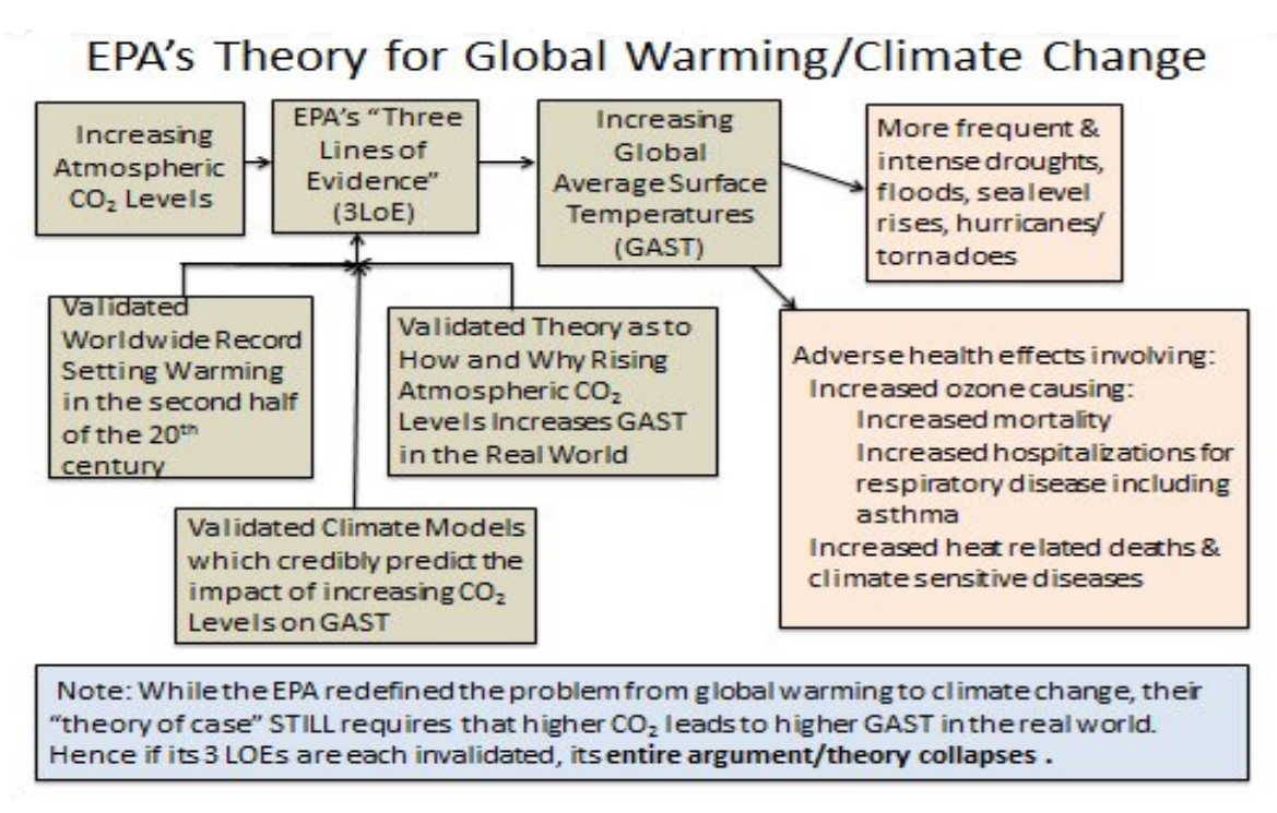
https://gizmodo.com/we-are-witnessing-a-new-brain-drain-as-scientists-flee-america-for-france-2000575654

This isn’t the first time France has pulled a stunt like this.

French President Offers US Climate Scientists €1.5 Million Each to Move to France

Despite generous French offers of financial support, last time France offered safe haven, many climate scientists stayed in the USA.

Perhaps this time things will be different, and all the alarmist climate scientists will move to Europe.

To be fair, France has a well-funded academic system, but that is pretty much where it stops. There is a reason France isn’t home to startups like Google and Facebook. High taxes and excessive regulations in France deter US style entrepreneurs and startups.

France makes no secret of their hostility towards large corporations. France and other European nations regularly slam “Anglo-Saxon capitalism”, by which they mean laissez-faire capitalism – a French position which is rather sad and historically inaccurate.

The very phrase “laissez-faire” is of course French, a phrase coined in the 17th century, back when French philosophers saw economic freedom as a path to liberation from feudalism and economic stagnation. The French sadly retreated from this glorious moment of near freedom, and in modern times have in my opinion re-instated elements of the ancient feudal system, which has created a tightly controlled command economy overseen by feudal bureaucrats, a straightjacketed form of capitalism where the French and European state is always firmly in control.

Despite all this, for scientists who never plan to ever do anything economically productive, France could be a good opportunity. Being a court philosopher in a feudal state is a well-paid job, so long as your philosophy pleases the lord.

You Almost Got It Right, New York Post, Subsidence Is Sinking Coastal Cities, Climate Change Isn’t Raising Seas

A recent New York Post (NYP) article, “Scary Map Reveals Major Coastal Cities Rapidly Sinking into Sea”, reports that a study from NASA claims that several major coastal cities are sinking at alarming rates due to a combination of land subsidence and rising sea levels. The NYP specifically mentions sea level problems in New York City, San Francisco, Los Angeles, and other cities, suggesting that their problems are due to a combination of subsidence and rising seas, the latter exacerbated by climate change. The latter point is misleading. Land subsidence is a well-documented problem in some cities, largely driven by local human activities such as groundwater extraction, poor urban planning, and natural geological processes.

From ClimateRealism

By Anthony Watts

A recent New York Post (NYP) article, “Scary Map Reveals Major Coastal Cities Rapidly Sinking into Sea”, reports that a study from NASA claims that several major coastal cities are sinking at alarming rates due to a combination of land subsidence and rising sea levels. The NYP specifically mentions sea level problems in New York City, San Francisco, Los Angeles, and other cities, suggesting that their problems are due to a combination of subsidence and rising seas, the latter exacerbated by climate change. The latter point is misleading. Land subsidence is a well-documented problem in some cities, largely driven by local human activities such as groundwater extraction, poor urban planning, and natural geological processes. Subsidence is not due to climate change. However, despite NASA’s claim, long-term sea-level rise trend data does not support claims that seas are rising at historically unusual rates. In fact, seas have been rising at a modest and steady rate for over a century, with no significant acceleration linked to human-caused emissions.

“In many parts of the world, like the reclaimed ground beneath San Francisco, the land is moving down faster than the sea itself is going up,” writes Marin Govorcin, the lead author of the NASA study. who specializes in remote sensing at NASA’s Propulsion Laboratory.”

Commenting on the study, Alexander Handwerger, another researcher at NASA’s Jet Propulsion Laboratory said, “The speed is more than enough to put human life and infrastructure at risk.”

“Accounting for this descent, sea levels — which are on the rise due to climate change — could creep up more than twice as much as previously forecast in Los Angeles and San Francisco in 25 years,” the NYP commented, but the key to the statement and the study itself is land subsidence, not rising seas.

Land subsidence is a localized issue caused primarily by excessive groundwater extraction, infrastructure issues, sediment compaction, and tectonic shifts. Climate change is not a factor in subsidence.

The study, published in Science Advances, cites short term data from satellites to imply that global sea-level rise is accelerating, an implication the NYP fails to question. However, real-world tide gauge data does not support this claim.

Long-term records from tide gauges—considered the gold standard for measuring local sea-level changes—show no evidence of unusual acceleration.

For example, NOAA’s tide gauge data from New York City’s Battery Park station, which has recorded sea levels since 1856, shows a steady rise of about 2.85 millimeters per year—a rate that has remained consistent for more than a century. This aligns closely with global tide gauge records, which show that average sea levels have been rising at a rate of 1-3 millimeters per year since the 1800s. Importantly, this gradual rise is not accelerating, despite increasing CO₂ emissions over the past several decades. See Figure 1 below:

Figure 1: Tide gauge derived plot of sea level trend since 1856 for New York City. The relative sea level trend is 2.94 millimeters/year with a 95% confidence interval of +/- 0.09 mm/yr based on monthly mean sea level data from 1856 to 2024 which is equivalent to a change of 0.96 feet in 100 years. Source: NOAA Tides and Currents.

Similarly, tide gauges in San Francisco show a steady sea level rise trend that is even lower than that found in New York City. (See Figure 2, below)

Figure 2: The relative sea level trend is 1.98 millimeters/year with a 95% confidence interval of +/- 0.17 mm/yr based on monthly mean sea level data from 1897 to 2024 which is equivalent to a change of 0.65 feet in 100 years. Source: NOAA Tides and Currents

Los Angeles’s rate of sea level rise, shown in Figure 3 below, is lower and slower still.

Figure 3: The relative sea level trend is 1.05 millimeters/year with a 95% confidence interval of +/- 0.21 mm/yr based on monthly mean sea level data from 1923 to 2024 which is equivalent to a change of 0.34 feet in 100 years. Source: NOAA Tides and Currents.

These three tide gauges from cities mentioned in the NYP article show no short- or long-term acceleration in sea level rise. Globally, in fact, there is little if any acceleration of sea level rise as data presented in Climate at a Glance: Sea Level Rise, demonstrates. Even if recent increases in the rate of rise recorded by some satellites are fully attributable to man-made climate change, it adds only 0.3 inch per decade more to the preexisting historic trend, and is still lower than the rate of rise that has occurred across many periods since the Earth entered its most recent interglacial 18,000 to 12,000 years before present.

Recent modest sea level trends contradict claims that climate change is making sea levels rise at “scary” and accelerated rates. In fact, multiple studies have shown that sea-level rise has remained relatively constant since the end of the Little Ice Age in the 19th century, here, here, here, and here, for example. If greenhouse gas emissions were truly driving an acceleration, we would expect to see a sharp upward trend in tide gauge records over the past 50 years—but we don’t.

A 2022 study highlighted in Climate Realism found that media claims of accelerating sea-level rise are often based on cherry-picked satellite data that fails to align with ground-based tide gauge measurements.

By conflating land subsidence with sea-level rise, all too often media outlets like the NYP mislead the public into believing that climate change is primarily or even solely responsible for coastal flooding threats. This is scientifically inaccurate and distracts from the real issues with subsidence that cities face. By focusing their efforts on the causes of land subsidence, such as ground water extraction issues, and compaction of unstable soil and fill used to add land to city oceanfront, rather than being distracted by the minimal or non-existent role greenhouse gas emissions are having in on sea level rise, policy makers could have far more direct and substantial impact on preventing flooding and losses.

The New York Post got the story half right. Its reporting would have been better had it eschewed any mention of climate change as a factor in the problems facing certain coastal cities.

Day: March 17, 2025

2025 The Poisonous Tree of Climate Change

Background on the Legal Precedents

2025 The Legal Landscape Has Shifted For EPA

The Bottom Line For Zeldin And EPA

Like this:

EPA questions 31 major energy regulations

Like this:

Germany’s First Offshore Wind Farm to Be Dismantled After Just 15 Years of Operation

Like this:

Trial of Mann v. Steyn: Post-Trial Motions Edition

Like this:

Trump Energy Choices Saving America from Economic Disaster

Like this:

EU Renewable Trends

Like this:

The Earth without Greenhouse Gases

Problems with the flat Earth model

A GHG-free spherical, rotating Earth model

The assumptions used in the model

The problems with the model

Discussion of what I learned

Future

Bibliography

Like this:

US Brain Drain: Climate Scientist Refugees are Fleeing to France?

Like this:

You Almost Got It Right, New York Post, Subsidence Is Sinking Coastal Cities, Climate Change Isn’t Raising Seas

Like this: