Global warming, climate change, all these things are just a dream come true for politicians. I deal with evidence and not with frightening computer models because the seeker after truth does not put his faith in any consensus. The road to the truth is long and hard, but this is the road we must follow. People who describe the unprecedented comfort and ease of modern life as a climate disaster, in my opinion have no idea what a real problem is.
Any manufacturer that does not have enough allowances, one way or another, will have to pay a fine of £15000. Manufacturers with excess allowances will therefore be able to sell these at close to £15000, as demand will almost certainly exceed supply. (This assumes that total EV sales are less than target, which seems highly probable).
As I reported a a couple of months ago, the Government has confirmed that the mandate cannot be legally imposed on foreign manufacturers. Their response was that they hoped the likes of BMW would simply comply!
But what about foreign manufacturers who export EVs to the UK? Would they be awarded allowances?
I asked the DfT, and this is their reply:
It could not be clearer then. If Tesla or one of the Chinese EV makers export to the UK, they will be given allowances which they can sell to UK manufacturers.
Chinese owned MG and Polestar, for instance, sold 34,000 EVs in this country last year. So their allowances would be worth £510 million. Tesla’s sales of the Y and 3 models totalled 49,000, worth £735 million
And with China already the world’s leading car exporter, and Chinese owned BYD challenging Tesla in global sales, these figures will quickly shoot up.
The cost will fall on UK car manufacturers, and probably end up being passed on to car buyers. The AA has already indicated that carmakers would cap the number of non-electric cars they sell, in order to hit the target. This will inevitably force prices up.
Funny, but I don’t recall voting to send billions in subsidies to China!
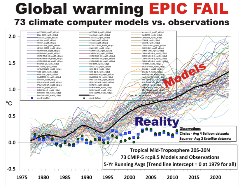
The only reason to object to the way we plot temperature time series is to Hide The Incline* in the long-term warming discrepancies between models and observations when showing the data on graphs.
Since Gavin Schmidt appears to have dug his heels in regarding how to plot two (or more) temperature times series on a graph having different long-term warming trends, it’s time to revisit exactly why John Christy and I now (and others should) plot such time series so that their linear trend lines intersect at the beginning.
While this is sometimes referred to as a “choice of base period” or “starting point” issue, it is crucial (and not debatable) to note it is irrelevant to the calculated trends. Those trends are the single best (although imperfect) measure of the long-term warming rate discrepancies between climate models and observations, and they remain the same no matter the base period chosen.
Again, I say, the choice of base period or starting point does not change the exposed differences in temperature trends (say, in climate models versus observations). Those important statistics remain the same.
The only reason to object to the way we plot temperature time series is to Hide The Incline* in the long-term warming discrepancies between models and observations when showing the data on graphs.
[*For those unfamiliar, in the Climategate email release, Phil Jones, then-head of the UK’s Climatic Research Unit, included the now-infamous “hide the decline” phrase in an e-mail, referring to Michael Mann’s “Nature trick” of cutting off the end of a tree-ring based temperature reconstruction (because it disagreed with temperature observations), and spliced in those observations in order to “hide the decline” in temperature exhibited by the tree ring data.]
I blogged on this issue almost eight years ago, and I just re-read that post this morning. I still stand by what I said back then (the issue isn’t complex).
Today, I thought I would provide a little background, and show why our way of plotting is the most logical way. (If you are wondering, as many have asked me, why not just plot the actual temperatures, without being referenced to a base period? Well, if we were dealing with yearly averages [no seasonal cycle, the usual reason for computing “anomalies”], then you quickly discover there are biases in all of these datasets, both observational data [since the Earth is only sparsely sampled with thermometers, and everyone does their area averaging in data-void infilling differently], and the climate models all have their own individual temperature biases. These biases can easily reach 1 deg. C, or more, which is large compared to computed warming trends.)
Historical Background of the Proper Way of Plotting
Years ago, I was trying to find a way to present graphical results of temperature time series that best represented the differences in warming trends. For a long time, John Christy and I were plotting time series relative to the average of the first 5 years of data (1979-1983 for the satellite data). This seemed reasonably useful, and others (e.g. Carl Mears at Remote Sensing Systems) also took up the practice and knew why it was done.
Then I thought, well, why not just plot the data relative to the first year (in our case, that was 1979 since the satellite data started in that year)? The trouble with that is there are random errors in all datasets, whether due to measurement errors and incomplete sampling in observational datasets, or internal climate variability in climate model simulations. For example, the year 1979 in a climate model simulation might (depending upon the model) have a warm El Nino going on, or a cool La Nina. If we plot each time series relative to the first year’s temperature, those random errors then impact the entire time series with an artificial vertical offset on the graph.
The same issue will exist using the average of the first five years, but to a lesser extent. So, there is a trade-off: the shorter the base period (or starting point), the more the times series will be offset by short-term biases and errors in the data. But the longer the base period (up to using the entire time series as the base period), the difference in trends is then split up as a positive discrepancy late in the period and a negative discrepancy early in the period.
I finally decided the best way to avoid such issues is to offset each time series vertically so that their linear trend lines all intersect at the beginning. This minimizes the impact of differences due to random yearly variations (since a trend is based upon all years’ data), and yet respects the fact that (as John Christy, an avid runner, told me), “every race starts at the beginning”.
In my blog post from 2016, I presented this pair of plots to illustrate the issue in the simplest manner possible (I’ve now added the annotation on the left):
Contrary to Gavin’s assertion that we are exaggerating the difference between models and observations (by using the second plot), I say Gavin wants to deceptively “hide the incline” by advocating something like the first plot. Eight years ago, I closed my blog post with the following, which seems to be appropriate still today: “That this issue continues to be a point of contention, quite frankly, astonishes me.”
The issue seems trivial (since the trends are unaffected anyway), yet it is important. Dr. Schmidt has raised it before, and because of his criticism (I am told) Judith Curry decided to not use one of our charts in congressional testimony. Others have latched onto the criticism as some sort of evidence that John and I are trying to deceive people. In 2016, Steve McIntyre posted an analysis of Gavin’s claim we were engaging in “trickery” and debunked Gavin’s claim.
In fact, as the evidence above shows, it is our accusers who are engaged in “trickery” and deception by “hiding the incline”.
It’s time we stopped messing around. Clearly, fossil fuels are feeding the world, greening the land, and boosting tree growth. Anyone who gives a damn about the environment needs to start campaigning to increase our fossil fuel emissions.
It’s time we stopped messing around. Clearly, fossil fuels are feeding the world, greening the land, and boosting tree growth. Anyone who gives a damn about the environment needs to start campaigning to increase our fossil fuel emissions.
Recently a batch of studies announced that the era of global greening might be over, or that drought stress might be browning the Earth faster than it was being greened. But a new study shows that the Earth is not only still getting greener, but that the rate of green growth is accelerating on more than half of the world.
Chen et al used four satellite datasets to estimate the Leaf Area Index (LAI). They found the long feared desertification of Earth is only accelerating over 7% of the globe while the long ignored greening is not increasing but even accelerating over 55% of the Earth. At this rate, the barren corners of the Earth are in danger of going missing.
Obviously, the habitat of koalas is benefiting hugely from coal, gas and petrol. But to be more serious, so are the worlds poor. If we care about the children of Haiti, we have a duty to liberate that coal, burn that oil and free up those stores of diesel.
Do it for the children…
All over the world, the dominant driver (according to the paper) was nearly always CO2.
CO2 fertilization is still the dominant (75.63%) driver of the trends on Earth in the last 20 years.
A website called Counterpunch.com ran a story on January 31st saying that we must solve climate change or disaster will befall us. The story is titled, “Solving Climate Change…or Else!” by Stan Cox. As we’ve written time and again on Climate Realism, these sorts of claims about worsening disasters are easily proven false simply by looking at historical data. The story cites other sources such as the New York Times but has no new information itself.
A website called Counterpunch.com ran a story on January 31st saying that we must solve climate change or disaster will befall us. The story is titled, “Solving Climate Change…or Else!” by Stan Cox. As we’ve written time and again on Climate Realism, these sorts of claims about worsening disasters are easily proven false simply by looking at historical data. The story cites other sources such as the New York Times but has no new information itself.
The story leads with this claim:
In December, the New York Timesreported that “Earth is finishing up its warmest year in the past 174 years and very likely the past 125,000.” (Though it’s not the Times’s style, that latter figure should have had a couple of exclamation points after it!) Furthermore, according to the National Oceanic and Atmospheric Administration’s chief scientist, “Not only was 2023 the warmest year in NOAA’s 174-year climate record — it was the warmest by far.”
Then after establishing what they believed to be a record warm year, they immediately go towards trying to link catastrophes to the warmth in 2023 without any real evidence to support it.
And you don’t have to wait for the distant future to see the impact of such accelerated heating. Just look at current global data. Comparing 2023 to 2022, the United Nations Office for the Coordination of Humanitarian Affairs (OCHA) reported a worldwide rise of 60% in the number of deaths from landslides, 278% from wildfires, and 340% from storms.
First, the landslides claim. Landslides aren’t a direct result of climate change, but rather are a symptom of weather events, such as excess rainfall saturating the ground and weakening it. Put simply, weather events are not climate. The following table is from Chapter 12 of the UN IPCC Sixth Assessment Report, Page 90 of Chapter 12 Climate Change Information for Regional Impact and for Risk Assessment. It essentially charts the UN IPCC’s assessment of the odds that each type of extreme weather is due to climate change.
Second, the increased wildfires and storms claim made by counterpunch.com are also addressed by the IPCC in the table below.
Table 1 from Page 90 – Chapter 12 of the UN IPCC Sixth Assessment Report. Emergence of Climate Impact Drivers (CIDs) in time periods, for the present-day, 2050, and 2100. The color corresponds to the confidence of the region with the highest confidence: white colors indicate where evidence of a climate change signal is lacking or the signal is not present, leading to overall low confidence of an emerging signal.
As can be seen from the table, there is no evidence of any increase or decrease, globally or by region, in the frequency, severity or extent of frost, mean precipitation, river floods, heavy precipitation and pluvial floods, landslides, aridity, hydrological drought, agricultural or ecological drought, fire weather or wildfires, mean wind speed, severe wind storms or tornados, tropical cyclones or hurricanes, sand and dust storms, snow glacial or ice sheets, heavy snowfall and ice storms, hail, snow avalanche, relative sea levels, coastal floods, coastal erosion, marine heatwaves, ocean acidity, or air pollution weather.
In addition to no increase in landslides or wildfires, the IPCC states there’s no increase in storms overall.
So, the “increasing disasters” claim made by counterpunch.com is completely nullified because there’s no evidence to support it whatsoever.
As for the claims of the hottest year ever in 2023 going back 125,000 years, that too is false. A study in 2013 by Marcott, et al. reconstructed temperatures from the present back to 11,300 years ago. Figure 2 shows clearly that temperatures about 9500 years ago known as the Holocene Climatic Optimum were warmer than present-day.
Figure 1: Temperature and carbon dioxide change during the Holocene. Black curve, global temperature reconstruction by Marcott et al., 2013. Red curve, CO2 levels as measured reported in Monnin et al., 2004. Importantly, Carbon Dioxide (CO2), in the red line, began increasing 8200 years ago even as temperatures, the black line, went down.
Clearly the author Stan Cox has no significant comprehension of climate data and climate history but prefers to simply regurgitate claims made in other publications as if they were fact. This lack of attention to detail and facts might explain why even after being online since 1993, counterpunch.com remains virtually unknown.
In its latest assessment, the North American Electric Reliability Corporation, a grid watchdog, warned that the MISO region is under some of the highest risks for resource inadequacy, which means that during peak demand periods, rolling blackouts are a possibility. Xcel Energy, according to the Energy News Network, is even looking at variable rates to encourage customers to conserve energy and use it during off-peak periods.
The South Dakota Public Utilities Commission told the utility that the “premature closure of these [coal] plants adds to the uncertainty of electrical generation resource adequacy in the upper Midwest.” Some energy experts call the government’s policies “irrational.”
Despite ongoing warnings that the electricity grid of the United States is becoming increasingly unstable, a major utility is moving forward with the elimination of two major coal-fired power plants in the upper Midwest. Energy analysts say the instability is a byproduct of the shutdown of reliable generation sources.
In its latest assessment, the North American Electric Reliability Corporation, a grid watchdog, warned that the MISO region is under some of the highest risks for resource inadequacy, which means that during peak demand periods, rolling blackouts are a possibility. Xcel Energy, according to the Energy News Network, is even looking at variable rates to encourage customers to conserve energy and use it during off-peak periods.
Michigan, Minnesota, Illinois and Nebraska have all set goals to decarbonize their grid by 2040 or 2050, which will mean eliminating coal-fired power plants entirely. These goals are on top of federal green energy mandates.
The Public is Blissfully Unaware–That Needs to Change
Some years ago, a weekly news program aired in the Netherlands on the subject Green Electrical Shocks. It employed images and humor to reveal electrical realities to an audience burdened with misconceptions. The video clip is below with English subtitles. For those who prefer reading, I provide the substantial excerpts from the program with my bolds.
How many of you have Green Electricity? I will estimate 69% And how much nationally? Oh, 69%! So we are very average, and in a good way, because the climate is very important.
Let me ask: Green electricity comes from . . .? Yes, electricity produced from windmills and solar panels. Nearly 2/3 of the Dutch are using it. That’s the image.
Well I have green news and bad news. The green news: Well done! The bad news: It is all one big lie. Time for the Green Electrical Shocks.
Shock #1: The green electricity from your socket is not green. When I switched to green electricity I was very proud. I thought, Yes, well done! The climate is getting warmer, but not any more thanks to me.
Well, that turned out to be untrue. All producers deliver to one communal grid. Green and grey electricity all mix. The electricity you use is always a mix of various sources. OK. It actually makes sense not to have separate green and grey cables for every house. So it means that of all electricity, 69% is produced in a sustainable way. But then:
Shock #2: Green Electricity is mostly fake. Most of the green electricity we think we use comes from abroad. You may think: So what. Green is green.
But that electricity doesn’t come from abroad, it stays abroad. If you have green electricity at home, it may mean nothing more than that your supplier has bought “green electricity certificates”.
In Europe green electricity gets an official certificate, Instead of selling on the electricity, they sell on those certificates. Norway, with its hydro power, has a surplus of certificates. Dutch suppliers buy them on a massive scale, while the electricity stays in Norway.
The idea was: if countries can sell those certificates, they can make money by producing more green electricity. But the Norwegians don’t produce more green electricity. But they do sell certificates.
The Dutch suppliers wave with those certificates, and say Look! Our grey electricity is green. Only one country has produced green electricity: Norway. But two countries take the credit. Norway, because they produce green electricity, and the Netherlands because, on paper, we have green electricity. Get it? That’s a nice deal.
More and more countries sell those certificates. Italy is now the top supplier. We buy fake green electricity from Italy, like some kind of Karma ham.
Now, let’s look again at the green electricity we all think we use. So the real picture isn’t 69%. If you cancel the certificates, only 21% of electricity is really green. Nowadays you can even order it separately if you don’t want to be part of that Norway certificates scam. You may think: 21% green is still quite a lot. But it is time for:
Shock #3: Not all energy is electricity. If you talk about the climate, you shouldn’t just consider electricity but all energy. When you look at all energy, like factories, cars, trains, gas fires, then the share of consumer electricity is virtually nothing. If you include everything in your calculation, it turns out that only 6% of all the energy we use in the Netherlands is green. It is a comedy, but wait:
Trees converted into pellets by means of petroleum powered machinery.
Shock #4: Most green energy doesn’t come from sun or wind, like you might think. Even the 6%, our last green hope, is fake. According to the CBS we are using more sun and wind energy, but most of the green energy is produced by the burning of biomass. Ah, more than half of the 6% green energy is biomass.
Ridiculous. What is biomass really? It is organic materials that we encounter every day. Like the content of a compost heap. How about maize leaves or hay? The idea behind burning organic materials is that it will grow up again. So CO2 is released when you burn it, but it will be absorbed again by new trees.
However, there is one problem. The forest grows very slowly and our power plants burn very fast. This is the fatal flaw in the thinking about biomass. Power plants burn trees too fast, so my solution: slow fire. Disadvantage: it doesn’t exist. So this is our next shock.
Shock#5: Biomass isn’t all that sustainable. It’s getting worse. There aren’t enough trees in the Netherlands for biomass. We can’t do it on our own. We don’t have enough wood, so we get it from America.
In the USA forests are cut at a high rate, Trees are shredded and compressed into pellets. These are shipped to the Netherlands and end up in the ovens of the coal plants. It’s a disaster for the American forests, according to environmental groups.
So we transport American forests on diesel ships to Europe. Then throw them in the oven because it officially counts as green energy. Only because the CO2 released this way doesn’t count for our total emissions.
In reality biomass emits more CO2 than natural gas and coal. These are laws of nature, no matter what European laws say. At the bottom line, how much sustainable energy do we really have in the Netherlands? Well, the only real green energy from windmills, solar panels etc. Is only 2.2%. of all the energy we use.
In Conclusion So the fact that 2/3 of the audience and of all Dutch people use green electricity means absolutely nothing. It’s only 2.2%, and crazier still, the government says it should be at 14% by 2020. They promised: to us, to Europe, to planet Earth: 14 instead of 2.2.
Instead of making a serious attempt to save the climate, they are only working on accounting tricks, like buying pieces of paper in Norway and burning American forests. They are only saving the climate on paper.
Summary Comment
As the stool above shows, the climate change package sits on three premises. The first is the science bit, consisting of an unproven claim that observed warming is caused by humans burning fossil fuels. The second part rests on impact studies from billions of research dollars spent uncovering any and all possible negatives from warming. And the third leg is climate policies showing how governments can “fight climate change.”
It is refreshing to see more and more articles by people reasoning about climate change/global warming and expressing rational positions. Increasingly, analysts are unbundling the package and questioning not only the science, but also pointing out positives from CO2 and warming. And as the Dutch telecast shows, ineffective government policies are also fair game.
Measured historical factors can be used to distinguish between urban and pristine stations.
Australian weather stations and data were tested. Australia’s low population density plus its many weather stations allow many “pristine” station candidates to be examined for studies of Urban Heat Island (UHI) effects.
From an initial list of 1,000+ stations, those with adequate data were narrowed down subjectively to 45 pristine station candidates. Some of their general properties are tabled below.
If several stations in a set are truly pristine, they should have similar temperature trends over time. If they do not have similar time series trends, then some factor more than natural variation must be affecting them; they cannot all be pristine.
Here is a graph of the trends of the 45 candidate stations.
This is for maximum temperatures, Tmax, years 1910 to 2020. In the following table, the linear least squares fit is calculated and expressed in the equivalent of ⁰C per century for maximum (Tmax), minimum (Tmin) and average (Tav) temperatures.
PRISTINE
Tmax trend 1910 to 2020
Tmin trend 1910 to 2020
Tav trend 1910 to 2020
RMS error Tmax
RMS error Tmin
BALLADONIA
0.2
0.6
0.4
6.6
4.99
BENCUBBIN
1.1
1.2
1.1
7.63
5.62
BIDYADANGA
2.0
1.9
1.9
3.52
5.08
BRUNETTE DNS
0.9
1.3
1.1
5.29
5.98
CAPE BORDA
2.4
1.1
1.7
4.64
3.21
CAPE BRUNY
1.6
1.4
1.5
4.05
2.96
CAPE CLEVELAND
0.1
2.9
1.5
3.37
3.15
CAPE LEEUWIN
0.9
0.7
0.8
3.37
2.89
CAPE MORETON
0.8
1.1
1.0
3.28
3.67
CAPE OTWAY
0.9
0.7
0.8
4.66
3.09
COCOS ISLAND
0.4
2.0
1.2
1.09
1.17
EDDYSTONE PT
1.4
1.1
1.2
3.59
3.49
ELLISTON
2.9
1.2
2.1
5.45
4.29
EMU CREEK
3.2
2.3
2.8
6.42
5.59
EUCLA
1.8
0.2
1.0
5.78
4.61
FLINDERS IS
1.7
1.6
1.6
4.35
4.39
GABO IS
1.4
0.3
0.9
3.48
3.49
HUME RESERVOIR
3.3
2.3
2.8
7.57
5.67
JERRYS PLAINS
3.1
1.0
2.1
6.21
5.91
KYANCUTTA
0.9
1.0
1.0
7.41
5.38
LADY ELLIOT IS
2.1
0.9
1.5
3.24
3.17
LARRIMAH
-0.3
1.5
0.6
3.69
5.33
LEARMONTH
3.1
0.8
2.0
5.72
5.04
LOCKHART R
1.5
2.4
1.9
2.24
2.79
LOW ISLES
1.0
0.8
0.9
2.98
2.17
MAATSUYKER IS
-0.1
1.3
0.6
3.79
2.68
MACQUARIE IS
1.0
0.9
1.0
1.99
2.53
MANDORAH
2.1
1.8
2.0
4.35
5.49
MANGALORE
2.6
0.6
1.6
7.28
5.33
MARDIE
0.8
3.1
1.9
5.01
5.47
MARRAWAH
1.5
1.5
1.5
3.72
3.07
MARREE
3.1
2.8
3.0
7.87
4.31
MONTAGUE IS
1.4
2.5
2.0
3.51
3.31
NEPTUNE IS
1.7
1.7
1.7
3.34
2.54
OENPELLI NT
0.4
1.7
1.0
2.52
3.16
OMEO VIC
0.5
1.6
1.1
6.78
5.02
PALMERVILLE
0.6
0.3
0.4
2.82
4.04
POINT HICKS
3.1
1.4
2.3
4.95
3.59
RABBIT FLAT
2.8
0.8
1.8
5.92
7.31
TABULAM
3.3
1.7
2.5
5.14
4.14
TARALGA
3.1
1.2
2.1
6.92
5.36
VICTORIA RIVER
0.8
0.4
0.6
4.16
6.21
WARMUN
0.4
0.5
0.5
4.39
5.52
WARRUWI
1.4
1.3
1.3
2.03
2.27
WILLIS ISLAND
0.4
1.0
0.7
1.99
1.77
Simple average
1.5
1.3
1.4
4.54
4.14
The linear trends for Tmax range from a high of 3.3 ⁰C per century at Hume Reservoir to a low of -0.3 ⁰C per century at Larrimah. These trends are far larger than the uniformity expected for true pristine sites with similar natural variation.
Therefore, the hypothesis that Measured historical factors can be used to distinguish between urban and pristine stations is shown to fail, because measured historical factors cannot even distinguish between one plausibly pristine station and another.
For wriggle matchers, here is the same data without the linear line of best fit, but with some lightly smoothed character retained.
The wriggles do not easily fall into a recognisable, simple, or systematic pattern. One might infer that there is “noise” from sources such as different start and end dates for the stations, plus station shifts at various dates, instrument changes, changes after quality testing and so on. Known system changes such as from ⁰F to ⁰C in November 1972 and from Liquid-In-Glass to Pt Resistance thermometry mostly in 1991 to 2001 have been studied for diverse stations. Their step changes if any are likely to be below 0.5 ⁰C, but the “noise” in these wriggles is an order of magnitude greater as shown by the RMS error figures tabled above in ⁰C units.
Willis Eschenbach has calculated a figure that can be compared with the wriggle graph above. It shows the expected earth surface temperatures derived from incoming radiation measured by the Ceres satellite system.
The trends from the Eschenbach graph using CERES data are about 1.5 ⁰C per century equivalent.
To the extent that comparison is valid – and I know of no reason to doubt – these satellite-based temperature estimates for random grid cells on the earth show time trends similar to each other and with matching wriggles over the last 20+ years. Something happens to the relation between the temperatures from satellite measurements and the land surface thermometer estimates we are discussing. Part of that “something” could be UHI, but my stations were chosen to have minimal UHI. How small is minimal? At Palmerville station,
“The same observer performed observations for 63 years from 1936 to 1999, and was the area’s sole remaining resident during the later part of that period. “
It is possible to create “adjusted temperatures” for these land surface stations. Most of the lighthouse stations in this candidate set have been separately adjusted by the ACORN-SAT procedures published by the Bureau of Meteorology. (A future article looks at the future for future adjustments).
Most past studies of Urban Heat Island effects start with this reasonable, logical, simple equation:
Tuhi = Turban – Tpristine
That framework works only if Turban and Tpristine can be measured. This article starts to show that there are impediments to the useful definition of Tpristine by measurement rather than by assignment. The next article in this series compares these 45 pristine candidate stations with 37 urban stations, to seek systematic differences between the two groups.
Through these articles, you are invited to consider if these temperature sets from Australia are much different to those from other countries, with the point in common that they are not fit for the purpose of influencing very expensive government policies.
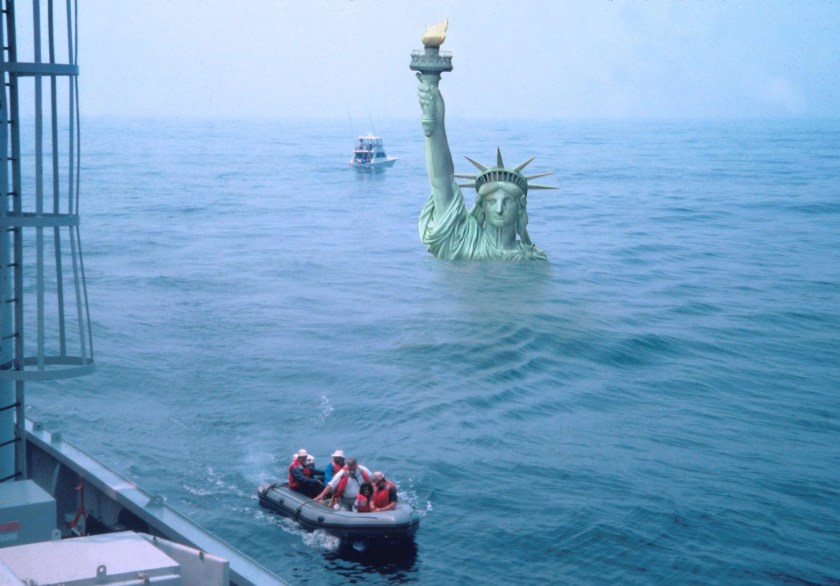
Such beach decorations exhibit the fervent belief of activists that sea levels are rising fast and will flood the coastlines if we don’t stop burning fossil fuels. As we will see below there is a concerted effort to promote this notion empowered with slick imaging tools to frighten the gullible.
Such beach decorations exhibit the fervent belief of activists that sea levels are rising fast and will flood the coastlines if we don’t stop burning fossil fuels. As we will see below there is a concerted effort to promote this notion empowered with slick imaging tools to frighten the gullible. Of course there are frequent media releases sounding the alarms. For example some examples already in 2024:
How rising sea levels will affect our coastal cities and towns Phys.org
Sea-level rise is here to stay and gathering pace, but the rate of future increase remains uncertain. It largely depends on what happens in Antarctica over the coming decades. This in turn depends on land and sea temperatures around the southern continent, which are directly linked to our efforts to limiting global warming to 1.5°C in line with the Paris Agreement. With over 250 million people now living on land less than 2 m above sea level, most in Asia, it is imperative we do everything we can to limit future sea-level rise.
Sea level rise could cost Europe billions in economic losses, study finds CBS News
Some regions of Europe could see “devastating” economic losses in the coming decades due to the rising oceans, researchers say. A new study found that under the worst-case scenario for emissions and sea level rise, the European Union and United Kingdom could lose 872 billion Euros (about $950 billion) by the end of this century, with many regions within them suffering GDP losses between 10% and 21%.
The study, published Thursday in the journal Scientific Reports, analyzed the economic impacts of sea level rise for 271 European regions. Researchers conducted their analysis based on estimates of high greenhouse gas emissions, which drive global temperature increases, a process that causes sea levels to rise.
Climate scientists project sea levels around New York City will rise by 1ft in 2030s alongside tropical storms and hotter temperatures Daily Mail
The New York City Panel on Climate Change (NPCC) released sea level projections that annual precipitation could increase by up to 10 percent over the years and warming would rise between two and 4.7 degrees Fahrenheit. The projection is part of a final report set to be released this spring. The estimates are based on carbon emissions and greenhouse gas emissions that cause ice caps to melt and increases precipitation, which leads to rising sea levels.
The rest of this post provides a tour of seven US cities demonstrating how the sea level scare machine promotes fear among people living or invested in coastal properties. In each case there are warnings published in legacy print and tv media, visual simulations powered by computers and desktop publishing, and a comparison of imaginary vs. observed sea level trends, updated with 2023 tidal gauge reports.
[Note: Some readers may be confused by the imagined sea level projections shown in red. These come from models that include IPCC suppositions in estimating sea level rise in various localities. For example, from the UCS (Union of Concerned Scientists):
A high scenario that assumes a continued rise in global carbon emissions and an increasing loss of land ice; global average sea level is projected to rise about 2 feet by 2045 and about 6.5 feet by 2100.
An intermediate scenario that assumes global carbon emissions rise through the middle of the century then begin to decline, and ice sheets melt at rates in line with historical observations; global average sea level is projected to rise about 1 foot by 2035 and about 4 feet by 2100.
A low scenario that assumes nations successfully limit global warming to less than 2 degrees Celsius (the goal set by the Paris Climate Agreement) and ice loss is limited; global average sea level is projected to rise about 1.6 feet by 2100.
The charts below also reflect sea level forecasts by state agencies like the California Coastal Commission]
Bath, the 8,500-resident “City of Ships,” is among the places in Maine facing the greatest risks from increased coastal flooding because so much of it is low-lying. The rising sea level in Bath threatens businesses along Commercial and Washington streets and other parts of the downtown, according to an analysis by Climate Central, a nonprofit science and journalism organization.
Water levels reached their highest in the city during a record-breaking storm in 1978 at a little more than 4 feet over pre-2000 average high tides, and Climate Central’s sea level team found there’s a 1-in-4 chance of a 5-foot flood within 30 years. That level could submerge homes and three miles of road, cutting off communities that live on peninsulas, and inundate sites that manage wastewater and hazardous waste along with several museums.
As global temperatures rise, so does the sea level. Experts predict it could rise as much as 20 inches by 2050, putting coastal communities, including those in Connecticut, in jeopardy.
One possible solution is a retreat from the shoreline, in which coastal homes are removed to take them out of imminent danger. This solution comes with many complications, including reductions in tax revenue for towns and potentially diminished real estate values for surrounding properties. Additionally, it can be difficult to get people to volunteer to relocate their homes.
Computer Simulations of the Future
Imaginary vs. Observed Sea Level Trends (2023 Update)
Could it be the end of the Blue Line as we know it? The Blue Line, which features a mile-long tunnel that travels underwater, and connects the North Shore with Boston’s downtown, is at risk as sea levels rise along Boston’s coast. To understand the threat sea-level rise poses to the Blue Line, and what that means for the rest of the city, we’re joined by WBUR reporter Simón Ríos and Julie Wormser, Deputy Director at the Mystic River Watershed Association.
As sea levels continue to rise, the Blue Line and the whole MBTA system face an existential threat. The MBTA is also facing a serious financial crunch, still reeling from the pandemic, as we attempt to fully reopen the city and the region. Joining us to discuss is MBTA General Manager Steve Poftak.
Computer Simulations of the Future
Imaginary vs. Observed Sea Level Trends (2023 Update)
Right now, of every US city, New York City has the highest population living inside a floodplain. By 2100, seas could rise around around the city by as much as six feet. Extreme rainfall is also predicted to rise, with roughly 1½ times more major precipitation events per year by the 2080s, according to a 2015 report by a group of scientists known as the New York City Panel on Climate Change.
But a two-degree warming scenario, which the world is on track to hit, could lock in dramatic sea level rise—possibly as much as 15 feet.
Computer Simulations of the Future
Imaginary vs. Observed Sea Level Trends (2023 Update)
NBC10 is looking at data and reading studies on climate change to showcase the impact. There are studies that show if the sea levels continue to rise at this rate, parts of Amtrak and Philadelphia International Airport could be underwater in 100 years.
Computer Simulations of the Future
Imaginary vs. Observed Sea Level Trends (2023 Update)
One 2018 Department of Transportation study has already found that a two-foot rise, expected by mid-century, would imperil a little more than five percent — 250-plus miles — of the state’s most high-traffic highways. That may not sound like a lot, but protecting those highways alone could easily cost several billion dollars. A Cat 5 hurricane could be far worse, with a fifth of the system vulnerable to flooding. The impact to seaports, airports and railroads — likely to also be significant and expensive — is only now under analysis.
Investigators are just beginning to try to unravel what caused the Champlain Towers South to collapse into a heap of rubble, leaving at least 159 people missing as of Friday. Experts on sea-level rise and climate change caution that it is too soon to speculate whether rising seas helped destabilize the oceanfront structure. The 40-year-old building was relatively new compared with others on its stretch of beach in the town of Surfside.
But it is already clear that South Florida has been on the front lines of sea-level rise and that the effects of climate change on the infrastructure of the region — from septic systems to aquifers to shoreline erosion — will be a management problem for years.
Computer Simulations of the Future
Imaginary vs. Observed Sea Level Trends (2023 Update)
As the sea rises, the land is also sinking: In the last century, the Texas coast sank about 2 feet into the sea, partly due to excessive groundwater pumping. Computer models now suggest that climate change will further lift sea levels somewhere between 1 and 6 feet over the next 50 years. Meanwhile, the Texas coastal population is projected to climb from 7 to 9 million people by 2050.
Protecting Galveston Bay is no simple task. The bay is sheltered from the open ocean by two low, sandy strips of land — Galveston Island and Bolivar Peninsula — separated by the narrow passage of Bolivar Roads. When a sufficiently big storm approaches, water begins to rush through that gap and over the island and peninsula, surging into the bay.
Computer Simulations of the Future
Imaginary vs. Observed Sea Level Trends (2023 Update)
Sea level rise is fueled by higher global temperatures that trigger two forces: Warmer water expands oceans while the increased temperatures hasten the melting of glaciers on Antarctica and Greenland and add yet more water to the oceans.
The California Ocean Protection Council, a branch of state government, forecasts a 1-in-7 chance that the average daily tides in the bay will rise 2 or more feet by 2070. This would cause portions of the marshes and bay trail in Hayward to be underwater during high tides. Add another 2 feet, on the higher end of the council’s projections for 2100 and they’d be permanently submerged. Highway 92 would flood during major storms. So would the streets leading into the power plant.
Along San Francisco’s Mission Creek, sea level rise unsettles the waters. Each section of this narrow channel must be tailored differently to meet an uncertain future. Do nothing, and the combination of heavy storms with less than a foot of sea level rise could send Mission Creek spilling over its banks in a half-dozen places, putting nearby housing in peril and closing the two bridges that cross the channel.
Whatever the response, we won’t know for decades if the city’s efforts can keep pace with the impact of global climatic forces that no local government can control.
Though Mission Creek is unique, the larger dilemma is one that affects all nine Bay Area counties.
Computer Simulations of the Future
Imaginary vs. Observed Sea Level Trends (2023 Update)
Summary: This is a relentless, high-tech communications machine to raise all kinds of scary future possibilities, based upon climate model projections, and the unfounded theory of CO2-driven global warming/climate change. The graphs above are centered on the year 2000, so that the 21st century added sea level rise is projected from that year forward. In addition, we now have observations at tidal gauges for the first 23 years, nearly 1/4 of the total expected. The gauges in each city are the ones with the longest continuous service record, and wherever possible the locations shown in the simulations are not far from the tidal gauge. For example, NYC best gauge is at the Battery, and Fulton St. is also near the Manhattan southern tip.
Already the imaginary rises are diverging greatly from observations, yet the chorus of alarm goes on. In fact, the added rise to 2100 from tidal gauges ranges from 6 to 9.5 inches, except for Galveston projecting 20.6 inches. Meanwhile models imagined rises from 69 to 108 inches. Clearly coastal settlements must adapt to evolving conditions, but also need reasonable rather than fearful forecasts for planning purposes.
Something unprecedented is happening in Earth orbit. In only a few short years, the satellite population has skyrocketed, more than doubling since 2020. In the past year alone, more satellites have been launched than during the first thirty years of the Space Age. Much of this activity is driven by SpaceX and its growing mega-constellation of Starlink internet satellites.
Feb. 1, 2024: Something unprecedented is happening in Earth orbit. In only a few short years, the satellite population has skyrocketed, more than doubling since 2020. In the past year alone, more satellites have been launched than during the first thirty years of the Space Age. Much of this activity is driven by SpaceX and its growing mega-constellation of Starlink internet satellites.
Environmentalists have raised many concerns about Starlink including light-pollution of the night sky, a potentially hazardous traffic jam in low-Earth orbit, and even ozone depletion. Copycat mega-constellations by other companies and countries will only multiply these concerns.
Now there’s a new reason to worry. According to a new study by Sierra Solter, megaconstellations could alter and weaken Earth’s magnetic field.
Solter is a graduate student at the University of Iceland, working on her PhD in plasma physics. She recently realized something overlooked by many senior colleagues: “More than 500,000 satellites are expected in decades ahead, primarily to build internet megaconstellations. Every satellite that goes up will eventually come down, disintegrating in Earth’s atmosphere. This will create a massive layer of conducting, electrically charged particles around our planet.”
To understand the scale of the problem, consider the following: If you gathered up every charged particle in Earth’s Van Allen Belts, their combined mass would be only 0.00018 kg. Other components of the magnetosphere such as the ring current and plasmasphere are even less massive. For comparison, “the mass of a second generation Starlink satellite is 1250 kilograms, all of which will become conductive debris when the satellite is eventually de-orbited,” says Solter.
Metal debris from a single deorbited Starlink satellite is 7 million times more massive than the Van Allen Belts. An entire megaconstellation is billions of times more massive. These ratios point to a big problem.
“The space industry is adding enormous amounts of material to the magnetosphere in comparison to natural levels of particulate matter,” says Solter. “Due to the conductive nature of the satellite debris, this may perturb or change things.”
There is already evidence of this process in action. A 2023 study by researchers using a high-altitude NASA aircraft found that 10% of aerosols in the stratosphere contain aluminum and other metals from disintegrating satellites and rocket stages. These particles are drifting down from “the ablation zone” 70 to 80 km above Earth’s surface where meteors and satellites burn up.
Solter decided to look for changes in the electrical properties of the ablation zone–and she found something. A NASA model of the upper atmosphere shows a sharp increase in the “Debye Length” just where satellites break apart when they deorbit:
“Debye Length” is a number that tells researchers how far an unbalanced electrical charge can be felt in conducting plasmas. The fact that it changes abruptly in the same place satellites disintegrate may be significant.
Extrapolating into the future, Solter worries that satellite debris could weaken Earth’s magnetic field–the same magnetic field that protects us from cosmic rays and solar storms.
“It’s a textbook undergraduate physics problem,” she explains. “Suppose you put a conductive shell (satellite debris) around a spherical magnet (Earth). Outside the shell, the magnetic field goes to zero due to shielding effects. This is a highly simplified comparison, of course, but we might actually be doing this to our planet.”
Solter’s preliminary study appears to show that the space industry is indeed perturbing the environment. “It is very concerning,” she concludes. “We absolutely cannot dump endless amounts of conductive dust into the magnetosphere and not expect some kind of impact. Multidisciplinary studies of this pollution are urgently needed.”
For more information, you can read Solter’s original research here.
Like rich nations have nothing better to do than discuss than giving big climate handouts to poor nations which have a shameful corruption index score.
Like rich nations have nothing better to do than discuss than giving big climate handouts to poor nations which have a shameful corruption index score.
For Cop29 to succeed, rich nations must get their parliaments to agree more finance now
Published on 30/01/2024, 2:49pm
Rich nations always say they need their parliaments approval for climate finance at Cops – now is the time to start
Although 2024 has just begun, the coming months will determine if Cop29 will be a success and whether benefits will trickle down to vulnerable communities in developing countries.
The Cop29 summit in Baku in November will focus on climate finance.
Government negotiators in the Global North always tell us that their ambition on finance depends on their parliaments.
…
They stress that they have no mandate, or possibility to scale up funds, as parliaments will not approve.
So, as parliamentarian debates about budgets and allocations begin early in the year, they need to act now.
…
Without more grant-based funding, our plans to adapt to climate change and cut emissions will not be implemented; our efforts to ensure green and sustainable growth and development will not be successful and our possibilities to address the growing threat of climate-related loss and damage will never occur.
…
Evans Njewa is the chair of the Least Developed Countries group and an official in Malawi’s environment ministry.
The author is “chair of the Least Developed Countries group”.
Why are those countries so undeveloped?
Malawi has lots of sunlight, good agricultural land and abundant rainfall in the wet season.
But there are problems in paradise. Transparency.org, which tracks global corruption, paints a bleak picture of Malawi corruption. 72% of surveyed locals thought corruption had increased in the last 12 months. 28% of public service users admitted they had paid a bribe.
From the Heritage Index of Economic Freedom :- Economic expansion remains fragile in the absence of a dynamic private sector. Malawi lags in competitiveness and promotion of the broad-based economic activity that is needed to reduce poverty. The poor quality of physical and legal infrastructure, made worse by the government’s inefficiency, is a serious impediment to long-term economic development.
Somehow I doubt a plane load of climate cash would help improve this situation.
Officials like Evans Njewa should put their energy into fixing Malawi’s domestic problems, to encourage more development, instead of demanding handouts from other countries.









You must be logged in to post a comment.