Ocean Fertilization: Dust to Bloom

Wind driven dust fertilizes the oceans by delivering iron and other micronutrients that stimulate phytoplankton growth, strengthen the biological carbon pump, and influence global climate. The core idea is that dust acts as a nutrient delivery system from land to sea, especially in regions where iron limits productivity.

From CO2 Coalition Substack

by Ganapathy Shanmugam, Ph.D.

We present evidence for Ocean Fertilization, using pattern recognition, with data from (1) the Sahara Desert, (2) the Taklamakan Desert, (3) the North Atlantic, (4) the Equatorial Atlantic, (5) the South Atlantic, (6) the Bay of Biscay, (7) the Strait of Hormuz, (8) the Bass Strait, (9) the Sea of Okhotsk, and (10) the Global Wind Circulation. Wind driven dust fertilizes the oceans by delivering iron and other micronutrients that stimulate phytoplankton growth, strengthen the biological carbon pump, and influence global climate. The core idea is that dust acts as a nutrient delivery system from land to sea, especially in regions where iron limits productivity.

Introduction

Pattern recognition, which we used in this study, is the ability to identify recurring structures, regularities, or relationships in data, signals, or experiences. It’s a fundamental principle in both human cognition and artificial intelligence, forming the basis of learning, problem-solving, and prediction. In this case, the sites where both wind-driven dust and phytoplankton blooms occur.

The Concept

Strong et al. (2009) note that the carbon dioxide that would otherwise be in the atmosphere is stored in the deep sea because the biological pump puts and keeps it there. Phytoplankton in the lighted

surface layer take up nutrients (e.g., nitrate and phosphate) and grow, converting CO2 to organic

matter that fuels marine food webs (Fig. 1).

The Problem

According to ACE (Antarctic Climate & Ecosystems) (2008), “While controlled iron fertilization

experiments have shown an increase in phytoplankton growth, and a temporary increase in drawdown of atmospheric CO2, it is uncertain whether this would increase carbon transfer into the deep ocean over the longer-term.” As illustrated by K. Buesseler of the Woods Hole Oceanographic Institution (Fig. 2), it is not yet known whether fertilization might generally enhance ecosystem production and drawdown of CO2 (in left panel), or whether this might lead to substantial and unwanted ecosystem changes that ultimately might diminish production and do little or nothing to enhance CO2 drawdown (right panel).

Furthermore, Hernández-León and Lichtfouse (2026) cautioned that many issues are yet to be investigated. For instance, the zooplankton burst that follows the phytoplankton bloom, and the carbon export by large fecal pellets remain poorly known (Fig. 3).

Also, it would be nice to be able to say which nutrient is responsible for the bloom, if it has been driven by iron (dust) alone or by other nutrients, such as phosphates, or nitrates for diatoms. Although we do not have answers to many questions, we must proceed with our efforts to gather data. We hope that this study will provide the incentives for young researchers who wish to explore this crucial climate issue.

The Evidence

We present a plethora of published data and images related to understanding Ocean Fertilization.

  • Knippertz (2014) provided a schematic depiction of a convective dust storm in the foothills of the Atlas Mountains in northwestern Africa (Fig. 4). The mountains serve as a trigger for deep moist convection. Evaporation on the dry Saharan side leads to evaporative cooling and the generation of a dust density current (Knippertz et al. 2007). Although developed for the Sahara Dust Storms, this model is applicable in general from a fluid mechanics viewpoint.

The Saharan Air Layer (SAL) has unique properties of warmth, dry air, and strong winds that can have significant moderating impacts on tropical cyclone formation and intensification. There are three characteristics of these Saharan dust outbreaks that can affect tropical cyclones, tropical disturbances, and the general climatology of the Atlantic tropical atmosphere: In the context of Ocean Fertilization, SAL carries large amount of dust across the Atlantic (Fig. 5).

The World’s deserts serve as the source of particles for dust storms. The Sahara Desert has an estmated area of 9.2 million km² (Fig. 6). Most dust storms originate from dry, disturbed soils, playas, agricultural lands, and alluvial deposits.

· Although sand dunes are an important component of a desert environment, such as the Taklamakan in NW China (Figs. 7 and 8), they are not major sources of particles for dust storms. The reason is that sand dunes are dominated by coarse sand, whereas fine silt and clay — the particles that create dust storms — are scarce.

In documenting the “Long-range transport of dust enhances oceanic iron bioavailability”, Kenlee et al. (202) (Fig. 9) evaluated the supply of wind-borne bioavailable Fe and its potential impact on Fe-based climate feedbacks over the last 120,000 years. They examined sediment profiles from four localities that define a proximal to distal transect relative to Saharan dust inputs. Bulk d56Fe isotope compositions (average = -0.05‰) and FeT/Al ratios suggest crustal values, which pointing to a dominant dust origin for the sediments at all four sites.

Satellite imagery shows that a 800-km long tongue of the Saharan dust storm penetrates into the Bay of Biscay with a phytoplankton bloom along the coast of France (Fig. 10). This occurrence of bloom near the tip of the dust storm is fortuitous.

· Blooms in the Strait of Hormuz resemble modern painting (Fig. 13). This area is constantly swept by dust storms.

In the Equatorial Atlantic, fertilizing the Amazon region (Fig. 14) with West African dust was discussed by Bristow et al. (2010). They presented the results of chemical analysis of 28 dust samples collected from the source area, which indicate that up to 6.5 Tg of Fe and 0.12 Tg of P are exported from the Bodélé Depression every year. This suggests that the Bodélé may be a more significant micronutrient supplier than previously proposed.

In the South Atlantic Ocean, the occurrence of dust storms and blooms Off Argentina is also striking (Shanmugam, 2018) (Fig. 15).

Dust and Bloom in the Bass Strait, between Australia and Tasmania (Fig. 16), have been documented.

  • Sea of OkhotskLeft Panel: Dust Tongue Length: 250 km (Fig. 17A)Right Panel: Bloom Ring Diameter: 200 km (Fig. 17B)

Finally, there is a general correlation between the Global Wind Circulation (Fig. 18A) and the Global Chlorophyll plumes (Fig. 18B).

CO2 Reality

By combining results of this study with earlier works on dust storms by Shanmugam (2026 and by Elias and Palmer (2016), we make some general inferences (Fig. 19).

They are:

1) Glacial Maxima

2) Low CO2

3) Low Vegetation

4) High Dust Production

5) High Ocean Fertilization

Furure Research

Core drivers of phytoplankton bloom formation are (Fig. 20):

  • Seed populations of phytoplankton already present in the water
  • Sufficient nutrients (nitrate, phosphate, silicate, iron)
  • Strong sunlight
  • Physical retention near the surface so cells stay in the euphotic zone.

In this article, We have addressed the role of just one nutrient (iron). There is much more research to be done.

Acknowledgements

I thank Angela Wheeler, Executive Director of the CO2 Coalition, for inviting me to present this contribution and Ethan Otte for helping. I also thank William Happer for valuable suggestions. I am grateful to Jean Shanmugam for her comments. I acknowledge with thanks the use of images from NASA, NOAA, WHOI, National Geographic, Elsevier, Springer, and Wikipedia.

References

ACE (Antarctic Climate & Ecosystems) (2008). Position Analysis: Ocean fertilisation: science and policy issues.19 p. https://web.whoi.edu/ocb-fert/wp-content/uploads/sites/100/2017/07/PA03_fertilisation_V2FIN_081008_56383.pdf

Bristow, C. S., K. A. Hudson-Edwards, and A. Chappell (2010), Fertilizing the Amazon and equatorial Atlantic with West African dust, Geophys. Res. Lett., 37, L14807, doi:10.1029/2010GL043486.

Chisholm, S.W. (2000). Stirring times in the Southern Ocean. Nature 407:685-686.

Elias, R. and Palmer, M. (2016). Modulation of ice ages via precession and dust-albedo feedbacks. Geoscience Frontiers, Volume 7, Issue 6, November 2016, Pages 891-909.

Hernández-León, S., Lichtfouse, E. (2026). Ocean iron fertilization for carbon dioxide removal and climate change mitigation. Environ Chem Lett (2026). https://doi.org/10.1007/s10311-026-01907-1

Kenlee, B., Owens, J. D., Raiswell, R., Poulton, S. W., Severmann, S., Sadler, P. M. and Lyons, T. W. (2024) Long-range transport of dust enhances oceanic iron bioavailability. Front. Mar. Sci. 11:1428621. doi: 10.3389/fmars.2024.1428621

Knippertz, P. (2014). Meteorological Aspects of Dust Storms. In: Knippertz, P., Stuut, JB. (eds) Mineral Dust. Springer, Dordrecht. https://doi.org/10.1007/978-94-017-8978-3_6

Knippertz P, Deutscher C, Kandler K et al (2007). Dust mobilization due to density currents in the Atlas region: Observations from the SAMUM 2006 field campaign. J Geophys Res 112, D21109, doi:10.1029/2007JD008774

Shanmugam, G. (2018). A global satellite survey of density plumes at river mouths and at other environments: plume configurations, external controls, and implications for deep-water sedimentation. Petrol. Explor. Development, 45(4), 640–661.

Shanmugam, G., (2026). Frequency of Dust Storms: Increases due to Climate Change (WHO, 2025) Vs Decreases due to Complex Factors in the Sahara-Sahel Region (Yeo et al., 2026)! 6 p. CO2 Coalition Sub stack. July 22, 2026. https://co2coalition.substack.com/p/frequency-of-dust-storms-increases

Strong, A.L., J.J. Cullen, and S.W. Chisholm. (2009). Ocean fertilization: Science, policy, and commerce. Oceanography 22(3):236–261, doi:10.5670/oceanog.2009.83.

Citation

Shanmugam, G., (2026). Ocean Fertilization: Dust to Bloom

17 p. CO2 Coalition Substack. August 10, 2026

Dr. Ganapathy Shanmugam is a CO2 Coalition Member, a petroleum geologist, and a sedimentologist with more than 50 years of experience in geology and energy research. He earned a Ph.D. from the University of Tennessee and worked for Mobil (1978-2000) before becoming an independent consultant. He has published extensively on deep-water sediments and petroleum reservoirs. His 318 published works on ResearchGate have reached 251,913 (over one-quarter million) reads from 32 countries as of August 10, 2026. He has also lectured and conducted workshops around the world.

Ocean Fertilization: From Dust to Bloom | Dr. Ganapathy Shanmugam

What’s New!

The CO2 Coalition has released its new episode of the Climate Debrief Podcast, The Forgotten Science of Preventing Wildfires, featuring Dr. Bob Zybach. Watch the full video on YouTube here!

The Climate Debrief Podcast is now also available on Apple, Spotify, Amazon, and iHeartRadio!

Godzilla Weather, Widespread Devastation & Economic Disruption

Will somebody save us all from these clowns who call themselves “journalists”?

From NOT A LOT OF PEOPLE KNOW THAT

By Paul Homewood

h/t Ian Magness

Will somebody save us all from these clowns who call themselves “journalists”?

Experts fear a ‘Godzilla’ El Niño will be strongest on record and cause widespread devastation.

The world could be on the brink of a “Godzilla-like” El Niño extreme weather pattern that could trigger economic and political disruption around the world.

El Niño, an oceanic heatwave that occurs two to three times each decade, is building in the Pacific around the equator, and is expected to peak in September, the United Nations’ World Meteorological Organization (WMO) has warned.

The warm current will affect weather patterns and increase the risk of droughts in Australia, and southern parts of Asia and Africa. It will also increase the likelihood of violent storms and heavy rainfall in parts of the Americas.

While droughts and storms are bad enough, experts say this could be the strongest El Niño on record, with even more severe potential outcomes. These include flooding, landslides, wildfires, famine, conflict and migration.

The expected severity has led to some meteorologists using the term Godzilla El Niño – after the colossal dinosaur-like creature that has featured in dozens of monster films.

El Niño has been causing weather-related disasters for centuries. It is thought to have contributed to the collapse of Peru’s ancient Moche civilisation in the eighth century, for example.

So, at a time when global supply chains and geopolitics are especially fragile, what could a Godzilla El Niño mean for the world? Here are three potential effects.

Read the full fairy tale here.

The report goes on to claim that food supply will be disrupted, migration will increase and and there will be “conflict zone flare-ups”.

All this from a weather phenomenon that comes around every four or five years – something humanity has managed to survive for millennia! Indeed, when you add in La Ninas, which also impact the weather, most years are “abnormal”!

El Ninos create a problem for the alarmist media. As global temperatures can rise by as much as a full degree in the space of a couple of years, as the climate swings from La Nina to El Nino, without any noticeable detriment to human life, why on earth should we be worried about much smaller rises in temperature spread over many decades?

Hence the attempts to frighten us with childish descriptions of Godzilla weather patterns triggering economic and political disruption around the world.

In reality, the changes to weather patterns brought about by El Nino have nothing at all to do with higher temperatures. They are the result of the change in atmospheric weather patterns.

The Met Office have this useful video, showing exactly what El Nino is:

Because of the changes in Pacific trade winds, as shown above, precipitation patterns around the world are also affected:

To label weather as “good” or “bad” is an oversimplification. The BBC, for instance, talk about floods in some regions, but heavier rain is more often than beneficial for agriculture.

But these effects tend to be much smaller than they would like us to believe. They are usually much more subtle. Take the Indian monsoon, for example:

Monsoon On Line

Yes, El Ninos tend to lead to droughts, but not always so. Droughts often occur in other years as well. But more significantly El Nino-linked droughts have not become more severe over time, which the silly Telegraph article implies. Indian rainfall patterns respond to atmospheric changes, not global temperatures.

Finally, just to deal with the food supply crisis, we are supposed to expect, the chart of cereal production proves that recent El Ninos have had zero effect on output:

FAOSTAT

I cant leave this without mentioning that the young reporter who wrote this twaddle is the Telegraph’s “Global Health Security Reporter”:

The Telegraph’s Global Health Security coverage is partly funded by the Bill & Melinda Gates Foundation.

Trees Get the Credit, But the Oceans Produce Most of Earth’s Oxygen

Trees and forests dominate the conversation about oxygen production, but the oceans are the planet’s primary oxygen factory.

AI generated by Grok

Trees and forests dominate the conversation about oxygen production, but the oceans are the planet’s primary oxygen factory.

Reliable sources, including NOAA and the Smithsonian, estimate that roughly 50% (or more) of Earth’s atmospheric oxygen is produced by the oceans. The main contributors are phytoplankton — microscopic drifting plants, algae, and cyanobacteria that perform photosynthesis in the sunlit upper ocean layer.

One single tiny species, Prochlorococcus, is responsible for up to 20% of all oxygen in the biosphere — more than all tropical rainforests combined.

Estimates sometimes range as high as 50–80% (or even 50–85% in some older popular accounts), depending on how net production is calculated.

Land plants and trees (including all forests) account for the remaining ~50%, with tropical rainforests contributing only about 28% in many assessments.

Important note: The oceans produce a huge amount of oxygen, but marine life (respiration and decomposition) also consumes roughly the same amount. The net contribution keeps the atmosphere balanced at ~21% oxygen over long timescales.

The imbalance in public attention comes down to simple visibility and messaging:

Trees are tall, photogenic, and easy to photograph or campaign around (“save the rainforest” resonates emotionally).

Phytoplankton are invisible to the naked eye — you can’t hug a bloom or plant one in your backyard.

Deforestation is a direct, visible human impact. Ocean threats (warming, stratification, nutrient changes) feel more abstract and global.

As one straightforward explanation puts it: phytoplankton “don’t have good PR” compared to charismatic trees.

Phytoplankton populations are sensitive to ocean warming, which can increase stratification and reduce nutrient upwelling.

Some recent modeling and field studies show regional shifts or modest declines in biomass in certain areas, and ocean deoxygenation is occurring (roughly 2% loss per decade in marine waters over recent decades).

However, the overall atmospheric oxygen level remains stable — the system has large buffers, and phytoplankton have shown resilience in past warm periods.

The oceans quietly do the heavy lifting for every other breath you take.

Protecting ocean health (reducing warming, pollution, and overfishing) is therefore one of the most effective ways to safeguard this invisible but essential oxygen engine.

There is a purely chemical (abiotic) way oxygen can be produced in the oceans — separate from photosynthesis by phytoplankton or trees.

This process is called “dark oxygen” production and was first reported in a 2024 study published in Nature Geoscience. It occurs in the deep sea, thousands of metres below the surface where no sunlight reaches.

Polymetallic nodules (potato-sized mineral lumps rich in manganese, nickel, cobalt, copper, and other metals) lie scattered across large areas of the abyssal seafloor, especially in the Clarion-Clipperton Zone of the Pacific.

These nodules can generate small electrical voltages (up to ~0.95 V measured on their surfaces, and potentially higher when clustered together).

The voltage is enough to drive seawater electrolysis — splitting water molecules (H₂O) into hydrogen gas (H₂) and oxygen gas (O₂) without any light or living organisms involved.

In lab and in-situ experiments, oxygen levels in sealed chambers rose significantly (sometimes more than tripling background concentrations) over two days when nodules were present.

The nodules essentially act like natural “geo-batteries,” with different metal layers creating an electrochemical potential that powers the reaction.

This chemical oxygen production is localized to the seafloor and does not contribute meaningfully to the global atmospheric oxygen we breathe (which is still overwhelmingly from surface phytoplankton photosynthesis). However, it could be important for:

Local oxygen supply to deep-sea life in otherwise oxygen-poor sediments.

Our understanding of how life might exist on other ocean worlds (e.g., icy moons like Europa or Enceladus).

It adds one more layer to why the oceans are far more chemically and biologically complex than the simple “trees produce oxygen” narrative suggests.

The discovery also ties into practical debates: the same nodules are targeted for deep-sea mining for battery metals, so any impact on this process is being carefully studied.

The Real Climate Science Crisis: CAGW Hypothesis Lacks Scientific Evidence

For a hypothesis to reach the status of being a legit theory, it requires withstanding the onslaught of observed empirical evidence. The CAGW hypothesis is no such animal.

Known by its more contemporary aliases, such as” climate crisis,” “climate emergency,” “climate collapse,” or “existential threat,” the CAGW has zero empirical evidence to support it.

From Science Matters

By Ron Clutz

From C3 headlines The Real Climate Science Crisis: The Catastrophic Anthropogenic Global Warming (CAGW) Hypothesis Is Without Scientific Evidence.  Excerpts in italics with my added images.

For a hypothesis to reach the status of being a legit theory, it requires withstanding the onslaught of observed empirical evidence. The CAGW hypothesis is no such animal.

Known by its more contemporary aliases, such as” climate crisis,” “climate emergency,” “climate collapse,” or “existential threat,” the CAGW has zero empirical evidence to support it.

Unlike the related hypothesis regarding greenhouse gases (GHG) and global warming, at least the GHG hypothesis has warming global temperature data that somewhat coincides with increasing atmospheric CO2 levels, putting aside the growing possibility that the purported cause-and-effect direction is probably the reverse.

In order to reach a CAGW climate disaster, global warming
temperatures must change rapidly in an accelerating manner
that will initiate a ‘tipping point’ for the climate.

The rapid acceleration would present its occurrence in a continuous increasing of the slope, i.e., trend, of temperatures, such as monthly temperatures. Each subsequent month would represent a greater temperature magnitude increase than the month before, hypothetically.

But those tipping point precursors are not occurring in the real-world climate.

For example, it is agreed by all climate scientists that oceans play a very major role in the world’s climate and its global temperatures due to their being both the world’s largest carbon sink and its largest heat content storage.

However, despite these characteristics, in totality, the global oceans HAVE NOT warmed since the year 2014. And certainly, there is no empirical evidence that oceans exhibit constant temperature increases of magnitude.

Quite the contrary, combined oceans exhibit a regular pattern of temperature decreases and increases, as the adjacent plot of NOAA’s monthly ocean data indicates.

Specifically, this is a plot (dark blue) of moving 5-year temperature changes ending each month of the 60-year period from March 1963 through March 2023.

[Explanation: the first data point is the temperature change for the 60 months ending on March 30, 1963; and the chart’s last temperature change data point is for the five 5 years (i.e. 60 months) ending on March 2023.]

The chart also includes a plot (green) of the moving 60-month CO2 level changes over the same sixty year period, plus a linear trend for both CO2 changes and ocean temperature changes.

The trend of the 60-month CO2 changes significantly exceeds the slight positive trend of ocean temperature changes by a factor of 117x. This huge differential undercuts the belief that global warming is primarily the result of GHGs. Which is confirmed by the paltry R^2 of +0.06 – an almost non-existent relationship between 5-year atmospheric CO2 changes and 5-year changes in ocean temperature.

Not only are the large increases in CO2 levels not causing a concerning uptick of temperature change magnitude, it also has not lead to any type of acceleration, per the linear trend since 1963.

Specifically, with a trend of a tiny +0.0001°C, that would project out 20 years to be an increase of 5-year temperature changes to an insignificant amount of +0.024°C – definitely not an existential threat of ‘runaway warming’ or a CAGW ‘climate crisis’ as portrayed by bureaucrats, politicians and Hollywood celebrities.

So, if 5 years of increasing amounts of CO2 in the atmosphere barely influence 5-year changes in temperature over a 60-year span, either in magnitude or acceleration rate, then it is highly unlikely that this trace gas would cause a catastrophic climate disaster or an extinction event.

Thus, it is fair to state that for all those scientists pushing a narrative of an imminent climate change catastrophe from CO2 without the requisite empirical evidence, this has become the real climate science crisis facing society.

Professor David King: We Must Consider Extreme Climate Solutions

“… Ideas such as thickening sea ice to prevent collapse … may once have seemed extreme. …”

From Watts Up With That?

Essay by Eric Worrall

“… Ideas such as thickening sea ice to prevent collapse … may once have seemed extreme. …”

We passed the 1.5C climate threshold. We must now explore extreme options

David King
Mon 7 Apr 2025 19.00 AEST

We do not have the luxury of rejecting solutions before we have thoroughly investigated their risks, trade-offs and feasibility

As a lifelong scientist, I have always believed that if something is possible, we can find a way to achieve it. And yet, one of the starkest realities we now face is that the world is failing to meet its climate goals. Last year marked a historic and deeply troubling threshold: for the first time, global temperatures exceeded 1.5C above pre-industrial levels. Without drastic and immediate climate action, this breach will not be temporary. The consequences – rising sea levels, extreme weatherand devastating loss of biodiversity – are no longer projections for the distant future. They are happening now, affecting millions of lives, and likely to cause trillions in damages in decades to come.

But we must think beyond our immediate horizons. When I read The Iliad, I am reminded that it was written 2,800 years ago. I often wonder: in another 2,800 years, what will people – if humanity as we know it still exists – read about our time? Will they see us as the generation that failed to act or one that made the choices necessary to safeguard the planet for the future?

…

One of the greatest challenges of climate science today is that many of the necessary levers to regain control are uncomfortable, even controversial. Ideas such as thickening sea ice to prevent collapse or brightening marine clouds to reflect sunlight may once have seemed extreme. Yet, as we contend with an escalating crisis, we must at least explore these possibilities. We do not have the luxury of rejecting solutions outright before we have thoroughly investigated their risks, trade-offs and feasibility.

…Read more: 

https://www.theguardian.com/commentisfree/2025/apr/07/climate-solutions-extreme-options

We hit 1.5C by some measures, but there are no climate disasters, except in the imagination of scientists like Professor David King. Nor will there be any climate disasters, even if temperatures climb higher.

Face it Professor King, you and your friends are wrong – a warmer world is a more benign world for humans.

The proof is that our monkey ancestors thrived in a much hotter world. The Palaeocene-Eocene Thermal Maximum, 5-8C hotter than today, was the age of monkeys. Our monkey ancestors thrived on the abundance of the hothouse PETM, and colonised much of the world, as far as Greenland and Siberia, only retreating when the cold returned.

The only thing I fear is our benign warm climate might soon come to an end – not in my lifetime, but way too soon for a human race which is only beginning to embrace its full potential.

Geologically the Earth is still locked in the Late Cenzoic Ice Age, which began 34 million years ago and still holds our planet in its frozen grip.

The last ice age was so cold it may have almost been an extinction event.

As we approach the end of the Holocene Interglacial, global cooling is a far greater long-term threat than global warming. Winter is coming, and we don’t have enough coal to drive back the ice.

February 2025 Oceans Keep Cool

El Nino is a phenomenon in the climate system that happens once every four or five years.  Heat builds up in the equatorial Pacific to the west of Indonesia and so on.  Then when enough of it builds up it surges across the Pacific and changes the currents and the winds.  As it surges toward South America it was discovered and named in the 19th century.  It is well understood at this point that the phenomenon has nothing to do with CO2.

From Science Matters

By Ron Clutz

The best context for understanding decadal temperature changes comes from the world’s sea surface temperatures (SST), for several reasons:

  • The ocean covers 71% of the globe and drives average temperatures.
  • SSTs have a constant water content, (unlike air temperatures), so give a better reading of heat content variations.
  • A major El Nino was the dominant climate feature in recent years.

HadSST is generally regarded as the best of the global SST data sets, and so the temperature story here comes from that source. Previously I used HadSST3 for these reports, but Hadley Centre has made HadSST4 the priority, and v.3 will no longer be updated.  HadSST4 is the same as v.3, except that the older data from ship water intake was re-estimated to be generally lower temperatures than shown in v.3.  The effect is that v.4 has lower average anomalies for the baseline period 1961-1990, thereby showing higher current anomalies than v.3. This analysis concerns more recent time periods and depends on very similar differentials as those from v.3 despite higher absolute anomaly values in v.4.  More on what distinguishes HadSST3 and 4 from other SST products at the end. The user guide for HadSST4 is here.

Note:  When doing monthly updates of HadSST4, it’s typical that values for the previous month or two will appear with slight adjustments.  However, this time there were scores of changed values scattered throughout the set and all values since 1979.  Strangely, the new values were in text format, so I needed to convert them to values in the spreadsheets.  Comparing the new and old datasets showed that the changes were mostly in the third decimal, and mostly negative (i.e. the adjusted value lower than the previous one.)  Overall, the global average anomaly since 1980 was lower by 0.01C.  The charts and analysis below are produced from the current data.

The Current Context

The chart below shows SST monthly anomalies as reported in HadSST3 starting in 2015 through February 2025. A global cooling pattern is seen clearly in the Tropics since its peak in 2016, joined by NH and SH cycling downward since 2016, followed by rising temperatures in 2023 and 2024.

Note that in 2015-2016 the Tropics and SH peaked in between two summer NH spikes.  That pattern repeated in 2019-2020 with a lesser Tropics peak and SH bump, but with higher NH spikes. By end of 2020, cooler SSTs in all regions took the Global anomaly well below the mean for this period.  A small warming was driven by NH summer peaks in 2021-22, but offset by cooling in SH and the tropics, By January 2023 the global anomaly was again below the mean.

Then in 2023-24 came an event resembling 2015-16 with a Tropical spike and two NH spikes alongside, all higher than 2015-16. There was also a coinciding rise in SH, and the Global anomaly was pulled up to 1.1°C last year, ~0.3° higher than the 2015 peak.  Then NH started down autumn 2023, followed by Tropics and SH descending 2024 to the present. After 10 months of cooling in SH and the Tropics, the Global anomaly came back down, led by NH cooling the last 4 months from its peak in August. It’s now about 0.1C higher than the average for this period. Note that the Tropical anomaly has cooled from 1.28C in 2024/01 to 0.72C as of 2025/2.

Comment:

The climatists have seized on this unusual warming as proof their Zero Carbon agenda is needed, without addressing how impossible it would be for CO2 warming the air to raise ocean temperatures.  It is the ocean that warms the air, not the other way around.  Recently Steven Koonin had this to say about the phonomenon confirmed in the graph above:

El Nino is a phenomenon in the climate system that happens once every four or five years.  Heat builds up in the equatorial Pacific to the west of Indonesia and so on.  Then when enough of it builds up it surges across the Pacific and changes the currents and the winds.  As it surges toward South America it was discovered and named in the 19th century.  It is well understood at this point that the phenomenon has nothing to do with CO2.

Now people talk about changes in that phenomena as a result of CO2 but it’s there in the climate system already and when it happens it influences weather all over the world.   We feel it when it gets rainier in Southern California for example.  So, for the last 3 years we have been in the opposite of an El Nino, a La Nina, part of the reason people think the West Coast has been in drought.

It has now shifted in the last months to an El Nino condition that warms the globe and is thought to contribute to this Spike we have seen. But there are other contributions as well.  One of the most surprising ones is that back in January of 2022 an enormous underwater volcano went off in Tonga and it put up a lot of water vapor into the upper atmosphere. It increased the upper atmosphere of water vapor by about 10 percent, and that’s a warming effect, and it may be that is contributing to why the spike is so high.

A longer view of SSTs

The graph below is noisy, but the density is needed to see the seasonal patterns in the oceanic fluctuations.  Previous posts focused on the rise and fall of the last El Nino starting in 2015.  This post adds a longer view, encompassing the significant 1998 El Nino and since.  The color schemes are retained for Global, Tropics, NH and SH anomalies.  Despite the longer time frame, I have kept the monthly data (rather than yearly averages) because of interesting shifts between January and July.

The graph above is noisy, but the density is needed to see the seasonal patterns in the oceanic fluctuations.  Previous posts focused on the rise and fall of the last El Nino starting in 2015.  This post adds a longer view, encompassing the significant 1998 El Nino and since.  The color schemes are retained for Global, Tropics, NH and SH anomalies.  Despite the longer time frame, I have kept the monthly data (rather than yearly averages) because of interesting shifts between January and July. 1995 is a reasonable (ENSO neutral) starting point prior to the first El Nino.

The sharp Tropical rise peaking in 1998 is dominant in the record, starting Jan. ’97 to pull up SSTs uniformly before returning to the same level Jan. ’99. There were strong cool periods before and after the 1998 El Nino event. Then SSTs in all regions returned to the mean in 2001-2.

SSTS fluctuate around the mean until 2007, when another, smaller ENSO event occurs. There is cooling 2007-8,  a lower peak warming in 2009-10, following by cooling in 2011-12.  Again SSTs are average 2013-14.

Now a different pattern appears.  The Tropics cooled sharply to Jan 11, then rise steadily for 4 years to Jan 15, at which point the most recent major El Nino takes off.  But this time in contrast to ’97-’99, the Northern Hemisphere produces peaks every summer pulling up the Global average.  In fact, these NH peaks appear every July starting in 2003, growing stronger to produce 3 massive highs in 2014, 15 and 16.  NH July 2017 was only slightly lower, and a fifth NH peak still lower in Sept. 2018.

The highest summer NH peaks came in 2019 and 2020, only this time the Tropics and SH were offsetting rather adding to the warming. (Note: these are high anomalies on top of the highest absolute temps in the NH.)  Since 2014 SH has played a moderating role, offsetting the NH warming pulses. After September 2020 temps dropped off down until February 2021.  In 2021-22 there were again summer NH spikes, but in 2022 moderated first by cooling Tropics and SH SSTs, then in October to January 2023 by deeper cooling in NH and Tropics.

Then in 2023 the Tropics flipped from below to well above average, while NH produced a summer peak extending into September higher than any previous year.  Despite El Nino driving the Tropics January 2024 anomaly higher than 1998 and 2016 peaks, following months cooled in all regions, and the Tropics continued cooling in April, May and June along with SH dropping.  After July and August NH warming again pulled the global anomaly higher, September through January 2025 resumed cooling in all regions, with a slight upward bump in February 2025.

What to make of all this? The patterns suggest that in addition to El Ninos in the Pacific driving the Tropic SSTs, something else is going on in the NH.  The obvious culprit is the North Atlantic, since I have seen this sort of pulsing before.  After reading some papers by David Dilley, I confirmed his observation of Atlantic pulses into the Arctic every 8 to 10 years.

Contemporary AMO Observations

Through January 2023 I depended on the Kaplan AMO Index (not smoothed, not detrended) for N. Atlantic observations. But it is no longer being updated, and NOAA says they don’t know its future.  So, I find that ERSSTv5 AMO dataset has current data.  It differs from Kaplan, which reported average absolute temps measured in N. Atlantic.  “ERSST5 AMO follows Trenberth and Shea (2006) proposal to use the NA region EQ-60°N, 0°-80°W and subtract the global rise of SST 60°S-60°N to obtain a measure of the internal variability, arguing that the effect of external forcing on the North Atlantic should be similar to the effect on the other oceans.”  So, the values represent SST anomaly differences between the N. Atlantic and the Global Ocean.

The chart above confirms what Kaplan also showed.  As August is the hottest month for the N. Atlantic, its variability, high and low, drives the annual results for this basin.  Note also the peaks in 2010, lows after 2014, and a rise in 2021. Then in 2023 the peak was holding at 1.4C before declining.  An annual chart below is informative:

Note the difference between blue/green years, beige/brown, and purple/red years.  2010, 2021, 2022 all peaked strongly in August or September.  1998 and 2007 were mildly warm.  2016 and 2018 were matching or cooler than the global average.  2023 started out slightly warm, then rose steadily to an  extraordinary peak in July.  August to October were only slightly lower, but by December cooled by ~0.4C.

Then in 2024 the AMO anomaly started higher than any previous year, then leveled off for two months declining slightly into April.  Remarkably, May showed an upward leap putting this on a higher track than 2023, and rising slightly higher in June.  In July, August and September 2024 the anomaly declined, and despite a small rise in October, ended close to where it began.  Now 2025 is starting much lower than the previous year.

The pattern suggests the ocean may be demonstrating a stairstep pattern like that we have also seen in HadCRUT4.

The purple line is the average anomaly 1980-1996 inclusive, value 0.17.  The orange line the average 1980-2024, value 0.38, also for the period 1997-2012. The red line is 2013-2024, value 0.67. As noted above, these rising stages are driven by the combined warming in the Tropics and NH, including both Pacific and Atlantic basins.

Curiosity:  Solar Coincidence?

The news about our current solar cycle 25 is that the solar activity is hitting peak numbers now and higher than expected 1-2 years in the future.  As live science put it:  Solar maximum could hit us harder and sooner than we thought. How dangerous will the sun’s chaotic peak be?  Some charts from spaceweatherlive look familar to these sea surface temperature charts.

Summary

The oceans are driving the warming this century.  SSTs took a step up with the 1998 El Nino and have stayed there with help from the North Atlantic, and more recently the Pacific northern “Blob.”  The ocean surfaces are releasing a lot of energy, warming the air, but eventually will have a cooling effect.  The decline after 1937 was rapid by comparison, so one wonders: How long can the oceans keep this up? And is the sun adding forcing to this process?

Footnote: Why Rely on HadSST4

HadSST is distinguished from other SST products because HadCRU (Hadley Climatic Research Unit) does not engage in SST interpolation, i.e. infilling estimated anomalies into grid cells lacking sufficient sampling in a given month. From reading the documentation and from queries to Met Office, this is their procedure.

HadSST4 imports data from gridcells containing ocean, excluding land cells. From past records, they have calculated daily and monthly average readings for each grid cell for the period 1961 to 1990. Those temperatures form the baseline from which anomalies are calculated.

In a given month, each gridcell with sufficient sampling is averaged for the month and then the baseline value for that cell and that month is subtracted, resulting in the monthly anomaly for that cell. All cells with monthly anomalies are averaged to produce global, hemispheric and tropical anomalies for the month, based on the cells in those locations. For example, Tropics averages include ocean grid cells lying between latitudes 20N and 20S.

Gridcells lacking sufficient sampling that month are left out of the averaging, and the uncertainty from such missing data is estimated. IMO that is more reasonable than inventing data to infill. And it seems that the Global Drifter Array displayed in the top image is providing more uniform coverage of the oceans than in the past.

USS Pearl Harbor deploys Global Drifter Buoys in Pacific Ocean

January 2025 Oceans Still Cool

The climatists have seized on this unusual warming as proof their Zero Carbon agenda is needed, without addressing how impossible it would be for CO2 warming the air to raise ocean temperatures.  It is the ocean that warms the air, not the other way around. 

From Science Matters

By Ron Clutz

The best context for understanding decadal temperature changes comes from the world’s sea surface temperatures (SST), for several reasons:

  • The ocean covers 71% of the globe and drives average temperatures;
  • SSTs have a constant water content, (unlike air temperatures), so give a better reading of heat content variations;
  • A major El Nino was the dominant climate feature in recent years.

HadSST is generally regarded as the best of the global SST data sets, and so the temperature story here comes from that source. Previously I used HadSST3 for these reports, but Hadley Centre has made HadSST4 the priority, and v.3 will no longer be updated.  HadSST4 is the same as v.3, except that the older data from ship water intake was re-estimated to be generally lower temperatures than shown in v.3.  The effect is that v.4 has lower average anomalies for the baseline period 1961-1990, thereby showing higher current anomalies than v.3. This analysis concerns more recent time periods and depends on very similar differentials as those from v.3 despite higher absolute anomaly values in v.4.  More on what distinguishes HadSST3 and 4 from other SST products at the end. The user guide for HadSST4 is here.

Note:  When doing monthly updates of HadSST4, it’s typical that values for the previous month or two will appear with slight adjustments.  However this time there were scores of changed values scattered throughout the set and all values since 1979.  Strangely, the new values were in text format, so I needed to convert them to values in the spreadsheets.  Comparing the new and old datasets showed that the changes were mostly in the third decimal, and mostly negative (i.e. the adjusted value lower than the previous one.)  Overall, the global average anomaly since 1980 was lower by 0.01C.  The charts and analysis below is produced from the current data.

The Current Context

The chart below shows SST monthly anomalies as reported in HadSST3 starting in 2015 through January 2025. A global cooling pattern is seen clearly in the Tropics since its peak in 2016, joined by NH and SH cycling downward since 2016, followed by rising temperatures in 2023 and 2024.

Note that in 2015-2016 the Tropics and SH peaked in between two summer NH spikes.  That pattern repeated in 2019-2020 with a lesser Tropics peak and SH bump, but with higher NH spikes. By end of 2020, cooler SSTs in all regions took the Global anomaly well below the mean for this period.  A small warming was driven by NH summer peaks in 2021-22, but offset by cooling in SH and the tropics, By January 2023 the global anomaly was again below the mean.

Now in 2023-24 came an event resembling 2015-16 with a Tropical spike and two NH spikes alongside, all higher than 2015-16. There was also a coinciding rise in SH, and the Global anomaly was pulled up to 1.1°C last year, ~0.3° higher than the 2015 peak.  Then NH started down autumn 2023, followed by Tropics and SH descending 2024 to the present. After 10 months of cooling in SH and the Tropics, the Global anomaly came back down, led by NH cooling the last 4 months from its peak in August. It’s now about 0.1C higher than the average for this period. Note that the Tropical anomaly has cooled from 1.28C in 2024/01 to 0.63C as of 2025/1.

Comment:

The climatists have seized on this unusual warming as proof their Zero Carbon agenda is needed, without addressing how impossible it would be for CO2 warming the air to raise ocean temperatures.  It is the ocean that warms the air, not the other way around.  Recently Steven Koonin had this to say about the phonomenon confirmed in the graph above:

El Nino is a phenomenon in the climate system that happens once every four or five years.  Heat builds up in the equatorial Pacific to the west of Indonesia and so on.  Then when enough of it builds up it surges across the Pacific and changes the currents and the winds.  As it surges toward South America it was discovered and named in the 19th century  It iswell understood at this point that the phenomenon has nothing to do with CO2.

Now people talk about changes in that phenomenon as a result of CO2 but it’s there in the climate system already and when it happens it influences weather all over the world.   We feel it when it gets rainier in Southern California for example.  So, for the last 3 years we have been in the opposite of an El Nino, a La Nina, part of the reason people think the West Coast has been in drought.

It has now shifted in the last months to an El Nino condition that warms the globe and is thought to contribute to this Spike we have seen. But there are other contributions as well.  One of the most surprising ones is that back in January of 2022 an enormous underwater volcano went off in Tonga and it put up a lot of water vapor into the upper atmosphere. It increased the upper atmosphere of water vapor by about 10 percent, and that’s a warming effect, and it may be that is contributing to why the spike is so high.

A longer view of SSTs

The graph below is noisy, but the density is needed to see the seasonal patterns in the oceanic fluctuations.  Previous posts focused on the rise and fall of the last El Nino starting in 2015.  This post adds a longer view, encompassing the significant 1998 El Nino and since.  The color schemes are retained for Global, Tropics, NH and SH anomalies.  Despite the longer time frame, I have kept the monthly data (rather than yearly averages) because of interesting shifts between January and July.

The graph above is noisy, but the density is needed to see the seasonal patterns in the oceanic fluctuations.  Previous posts focused on the rise and fall of the last El Nino starting in 2015.  This post adds a longer view, encompassing the significant 1998 El Nino and since.  The color schemes are retained for Global, Tropics, NH and SH anomalies.  Despite the longer time frame, I have kept the monthly data (rather than yearly averages) because of interesting shifts between January and July. 1995 is a reasonable (ENSO neutral) starting point prior to the first El Nino.

The sharp Tropical rise peaking in 1998 is dominant in the record, starting Jan. ’97 to pull up SSTs uniformly before returning to the same level Jan. ’99. There were strong cool periods before and after the 1998 El Nino event. Then SSTs in all regions returned to the mean in 2001-2.

SSTS fluctuate around the mean until 2007, when another, smaller ENSO event occurs. There is cooling 2007-8, a lower peak warming in 2009-10, following by cooling in 2011-12.  Again, SSTs are average 2013-14.

Now a different pattern appears.  The Tropics cooled sharply to Jan 11, then rise steadily for 4 years to Jan 15, at which point the most recent major El Nino takes off.  But this time in contrast to ’97-’99, the Northern Hemisphere produces peaks every summer pulling up the Global average.  In fact, these NH peaks appear every July starting in 2003, growing stronger to produce 3 massive highs in 2014, 15 and 16.  NH July 2017 was only slightly lower, and a fifth NH peak still lower in Sept. 2018.

The highest summer NH peaks came in 2019 and 2020, only this time the Tropics and SH were offsetting rather adding to the warming. (Note: these are high anomalies on top of the highest absolute temps in the NH.)  Since 2014 SH has played a moderating role, offsetting the NH warming pulses. After September 2020 temps dropped off down until February 2021.  In 2021-22 there were again summer NH spikes, but in 2022 moderated first by cooling Tropics and SH SSTs, then in October to January 2023 by deeper cooling in NH and Tropics.

Then in 2023 the Tropics flipped from below to well above average, while NH produced a summer peak extending into September higher than any previous year.  Despite El Nino driving the Tropics January 2024 anomaly higher than 1998 and 2016 peaks, following months cooled in all regions, and the Tropics continued cooling in April, May and June along with SH dropping.  After July and August NH warming again pulled the global anomaly higher, September and October resumed cooling in all regions.

What to make of all this? The patterns suggest that in addition to El Ninos in the Pacific driving the Tropic SSTs, something else is going on in the NH.  The obvious culprit is the North Atlantic, since I have seen this sort of pulsing before.  After reading some papers by David Dilley, I confirmed his observation of Atlantic pulses into the Arctic every 8 to 10 years.

Contemporary AMO Observations

Through January 2023 I depended on the Kaplan AMO Index (not smoothed, not detrended) for N. Atlantic observations. But it is no longer being updated, and NOAA says they don’t know its future.  So, I find that ERSSTv5 AMO dataset has current data.  It differs from Kaplan, which reported average absolute temps measured in N. Atlantic.  “ERSST5 AMO follows Trenberth and Shea (2006) proposal to use the NA region EQ-60°N, 0°-80°W and subtract the global rise of SST 60°S-60°N to obtain a measure of the internal variability, arguing that the effect of external forcing on the North Atlantic should be similar to the effect on the other oceans.”  So, the values represent SST anomaly differences between the N. Atlantic and the Global Ocean.

The chart above confirms what Kaplan also showed.  As August is the hottest month for the N. Atlantic, its variability, high and low, drives the annual results for this basin.  Note also the peaks in 2010, lows after 2014, and a rise in 2021. Then in 2023 the peak was holding at 1.4C before declining.  An annual chart below is informative:

Note the difference between blue/green years, beige/brown, and purple/red years.  2010, 2021, 2022 all peaked strongly in August or September.  1998 and 2007 were mildly warm.  2016 and 2018 were matching or cooler than the global average.  2023 started out slightly warm, then rose steadily to an extraordinary peak in July.  August to October were only slightly lower, but by December cooled by ~0.4C.

Then in 2024 the AMO anomaly started higher than any previous year, then leveled off for two months declining slightly into April.  Remarkably, May showed an upward leap putting this on a higher track than 2023, and rising slightly higher in June.  In July, August and September 2024 the anomaly declined, and despite a small rise in October, ended close to where it began.  Now 2025 is starting lower than the previous year.

The pattern suggests the ocean may be demonstrating a stairstep pattern like that we have also seen in HadCRUT4.

The purple line is the average anomaly 1980-1996 inclusive, value 0.17.  The orange line the average 1980-2024, value 0.38, also for the period 1997-2012. The red line is 2013-2024, value 0.67. As noted above, these rising stages are driven by the combined warming in the Tropics and NH, including both Pacific and Atlantic basins.

Curiosity:  Solar Coincidence?

The news about our current solar cycle 25 is that the solar activity is hitting peak numbers now and higher  than expected 1-2 years in the future.  As livescience put it:  Solar maximum could hit us harder and sooner than we thought. How dangerous will the sun’s chaotic peak be?  Some charts from spaceweatherlive look familar to these sea surface temperature charts.

Summary

The oceans are driving the warming this century.  SSTs took a step up with the 1998 El Nino and have stayed there with help from the North Atlantic, and more recently the Pacific northern “Blob.”  The ocean surfaces are releasing a lot of energy, warming the air, but eventually will have a cooling effect.  The decline after 1937 was rapid by comparison, so one wonders: How long can the oceans keep this up? And is the sun adding forcing to this process?

Footnote: Why Rely on HadSST4

HadSST is distinguished from other SST products because HadCRU (Hadley Climatic Research Unit) does not engage in SST interpolation, i.e. infilling estimated anomalies into grid cells lacking sufficient sampling in a given month. From reading the documentation and from queries to Met Office, this is their procedure.

HadSST4 imports data from gridcells containing ocean, excluding land cells. From past records, they have calculated daily and monthly average readings for each grid cell for the period 1961 to 1990. Those temperatures form the baseline from which anomalies are calculated.

In a given month, each gridcell with sufficient sampling is averaged for the month and then the baseline value for that cell and that month is subtracted, resulting in the monthly anomaly for that cell. All cells with monthly anomalies are averaged to produce global, hemispheric and tropical anomalies for the month, based on the cells in those locations. For example, Tropics averages include ocean grid cells lying between latitudes 20N and 20S.

Gridcells lacking sufficient sampling that month are left out of the averaging, and the uncertainty from such missing data is estimated. IMO that is more reasonable than inventing data to infill. And it seems that the Global Drifter Array displayed in the top image is providing more uniform coverage of the oceans than in the past.

USS Pearl Harbor deploys Global Drifter Buoys in Pacific Ocean

Oceans Rapidly Cooling UAH January 2025

The post below updates the UAH record of air temperatures over land and ocean. Each month and year expose again the growing disconnect between the real world and the Zero Carbon zealots.  It is as though the anti-hydrocarbon band wagon hopes to drown out the data contradicting their justification for the Great Energy Transition.  Yes, there was warming from an El Nino buildup coincidental with North Atlantic warming, but no basis to blame it on CO2.  

From Science Matters

By Ron Clutz

The post below updates the UAH record of air temperatures over land and ocean. Each month and year expose again the growing disconnect between the real world and the Zero Carbon zealots.  It is as though the anti-hydrocarbon band wagon hopes to drown out the data contradicting their justification for the Great Energy Transition.  Yes, there was warming from an El Nino buildup coincidental with North Atlantic warming, but no basis to blame it on CO2.  

As an overview consider how recent rapid cooling completely overcame the warming from the last 3 El Ninos (1998, 2010 and 2016).  The UAH record shows that the effects of the last one were gone as of April 2021, again in November 2021, and in February and June 2022.  At year end 2022 and continuing into 2023 global temp anomaly matched or went lower than average since 1995, an ENSO neutral year. (UAH baseline is now 1991-2020). Now we have had an usual El Nino warming spike of uncertain cause, unrelated to steadily rising CO2 and now dropping steadily.

For reference I added an overlay of CO2 annual concentrations as measured at Mauna Loa.  While temperatures fluctuated up and down ending flat, CO2 went up steadily by ~60 ppm, a 15% increase.

Furthermore, going back to previous warmings prior to the satellite record shows that the entire rise of 0.8C since 1947 is due to oceanic, not human activity.

gmt-warming-events

The animation is an update of a previous analysis from Dr. Murry Salby.  These graphs use Hadcrut4 and include the 2016 El Nino warming event.  The exhibit shows since 1947 GMT warmed by 0.8 C, from 13.9 to 14.7, as estimated by Hadcrut4.  This resulted from three natural warming events involving ocean cycles. The most recent rise 2013-16 lifted temperatures by 0.2C.  Previously the 1997-98 El Nino produced a plateau increase of 0.4C.  Before that, a rise from 1977-81 added 0.2C to start the warming since 1947.

Importantly, the theory of human-caused global warming asserts that increasing CO2 in the atmosphere changes the baseline and causes systemic warming in our climate.  On the contrary, all of the warming since 1947 was episodic, coming from three brief events associated with oceanic cycles. And now in 2024 we have seen an amazing episode with a temperature spike driven by ocean air warming in all regions, along with rising NH land temperatures, now dropping below its peak.

Chris Schoeneveld has produced a similar graph to the animation above, with a temperature series combining HadCRUT4 and UAH6. H/T WUWT

See Also Worst Threat: Greenhouse Gas or Quiet Sun?

January 2025 Ocean Leads Global Cooling

With apologies to Paul Revere, this post is on the lookout for cooler weather with an eye on both the Land and the Sea.  While you heard a lot about 2020-21 temperatures matching 2016 as the highest ever, that spin ignores how fast the cooling set in.  The UAH data analyzed below shows that warming from the last El Nino had fully dissipated with chilly temperatures in all regions. After a warming blip in 2022, land and ocean temps dropped again with 2023 starting below the mean since 1995.  Spring and Summer 2023 saw a series of warmings, continuing into October, followed by cooling in November and December.

UAH has updated their TLT (temperatures in lower troposphere) dataset for January 2025. Due to one satellite drifting more than can be corrected, the dataset has been recalibrated and retitled as version 6.1 Graphs here contain this updated 6.1 data.  Posts on their reading of ocean air temps this month are ahead of the update from HadSST4.  I posted recently on SSTs Ocean Even Cooler December 2024. These posts have a separate graph of land air temps because the comparisons and contrasts are interesting as we contemplate possible cooling in coming months and years.

Sometimes air temps over land diverge from ocean air changes. In July 2024 all oceans were unchanged except for Tropical warming, while all land regions rose slightly. In August we saw a warming leap in SH land, slight Land cooling elsewhere, a dip in Tropical Ocean temp and slightly elsewhere.  September showed a dramatic drop in SH land, overcome by a greater NH land increase. In October, ocean and land temps in both NH and Tropics dropped, pulling the global anomaly down. As was the case in November and December, now in January there was cooling everywhere, strongest in all ocean anomalies.

Note:  UAH has shifted their baseline from 1981-2010 to 1991-2020 beginning with January 2021.   v6.1 data was recalibrated also starting with 2021. In the charts below, the trends and fluctuations remain the same, but the anomaly values changed with the baseline reference shift.

Presently sea surface temperatures (SST) are the best available indicator of heat content gained or lost from earth’s climate system.  Enthalpy is the thermodynamic term for total heat content in a system, and humidity differences in air parcels affect enthalpy.  Measuring water temperature directly avoids distorted impressions from air measurements.  In addition, ocean covers 71% of the planet surface and thus dominates surface temperature estimates.  Eventually we will likely have reliable means of recording water temperatures at depth.

Recently, Dr. Ole Humlum reported from his research that air temperatures lag 2-3 months behind changes in SST.  Thus cooling oceans portend cooling land air temperatures to follow.  He also observed that changes in CO2 atmospheric concentrations lag behind SST by 11-12 months.  This latter point is addressed in a previous post Who to Blame for Rising CO2?

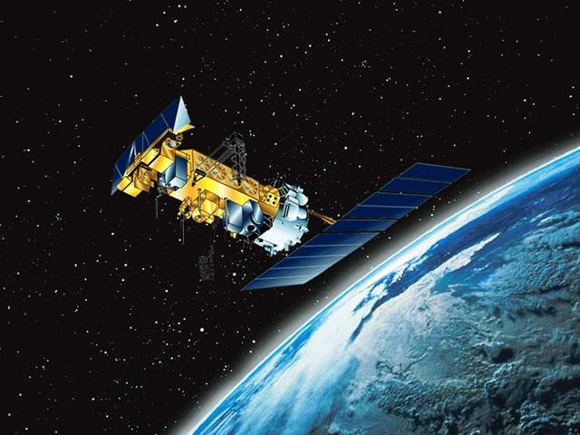
After a change in priorities, updates are now exclusive to HadSST4.  For comparison we can also look at lower troposphere temperatures (TLT) from UAHv6.1 which are now posted for January 2025.  The temperature record is derived from microwave sounding units (MSU) on board satellites like the one pictured above. Recently there was a change in UAH processing of satellite drift corrections, including dropping one platform which can no longer be corrected. The graphs below are taken from the revised and current dataset.

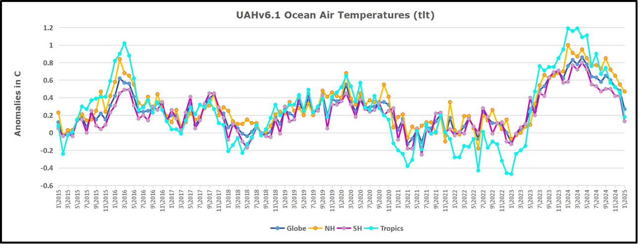
The UAH dataset includes temperature results for air above the oceans, and thus should be most comparable to the SSTs. There is the additional feature that ocean air temps avoid Urban Heat Islands (UHI).  The graph below shows monthly anomalies for ocean air temps since January 2015.

In 2021-22, SH and NH showed spikes up and down while the Tropics cooled dramatically, with some ups and downs, but hitting a new low in January 2023. At that point all regions were more or less in negative territory. 

After sharp cooling everywhere in January 2023, there was a remarkable spiking of Tropical ocean temps from -0.5C up to + 1.2C in January 2024.  The rise was matched by other regions in 2024, such that the Global anomaly peaked at 0.95C in May. Since then, all regions have cooled down sharply, Global anomaly dropping in January to 0.3C, as well as SH dropping down to 0.1C in January.

Land Air Temperatures Tracking in Seesaw Pattern

We sometimes overlook that in climate temperature records, while the oceans are measured directly with SSTs, land temps are measured only indirectly.  The land temperature records at surface stations sample air temps at 2 meters above ground.  UAH gives tlt anomalies for air over land separately from ocean air temps.  The graph updated for January is below.

Here we have fresh evidence of the greater volatility of the Land temperatures, along with extraordinary departures by SH land.  The seesaw pattern in Land temps is similar to ocean temps 2021-22, except that SH is the outlier, hitting bottom in January 2023. Then exceptionally SH goes from -0.6C up to 1.4C in September 2023 and 1.8C in  August 2024, with a large drop in between.  In November, SH and the Tropics pulled the Global Land anomaly further down despite a bump in NH land temps. December showed an upward rebound in SH and Tropics land temps, now offset by a dropping temps everywhere, pulling the Global land anomaly downward slightly.

The Bigger Picture UAH Global Since 1980

The chart shows monthly Global Land and Ocean anomalies starting 01/1980 to present.  The average monthly anomaly is -0.03, for this period of more than four decades.  The graph shows the 1998 El Nino after which the mean resumed, and again after the smaller 2010 event. The 2016 El Nino matched 1998 peak and in addition NH after effects lasted longer, followed by the NH warming 2019-20.   An upward bump in 2021 was reversed with temps having returned close to the mean as of 2/2022.  March and April brought warmer Global temps, later reversed

With the sharp drops in Nov., Dec. and January 2023 temps, there was no increase over 1980. Then in 2023 the buildup to the October/November peak exceeded the sharp April peak of the El Nino 1998 event. It also surpassed the February peak in 2016. In 2024 March and April took the Global anomaly to a new peak of 0.94C.  The cool down started with May dropping to 0.9C, and in June a further decline to 0.8C.  October went down to 0.7C,  November and December dropped to 0.6C. January down to 0.46C.

The graph reminds of another chart showing the abrupt ejection of humid air from Hunga Tonga eruption.

TLTs include mixing above the oceans and probably some influence from nearby more volatile land temps.  Clearly NH and Global land temps have been dropping in a seesaw pattern, nearly 1C lower than the 2016 peak.  Since the ocean has 1000 times the heat capacity as the atmosphere, that cooling is a significant driving force.  TLT measures started the recent cooling later than SSTs from HadSST4, but are now showing the same pattern. Despite the three El Ninos, their warming had not persisted prior to 2023, and without them it would probably have cooled since 1995.  Of course, the future has not yet been written.

Oceans Inhale and Exhale Carbon Dioxide, Since Forever

It could be that all the extra carbon dioxide in the atmosphere – the steady increase year on year, reported since 1958, despite all the airplanes grounded through covid it kept on increasing – is a consequence of the oceans breathing out a bit more, and nothing to do with you and me.

From Jennifer Marohasy

By jennifer

It could be that all the extra carbon dioxide in the atmosphere – the steady increase year on year, reported since 1958, despite all the airplanes grounded through covid it kept on increasing – is a consequence of the oceans breathing out a bit more, and nothing to do with you and me.

The amount of carbon sequestered in the oceans was meant to increase with the apparently significant increase in atmospheric levels because of industrialisation, except that observations, actual measurements, suggest that there has been no long-term increase.  The oceans might be breathing carbon dioxide in, and out, to their own rhythm that has nothing to do with you and me – or all the windfarms.

It could be that mankind is irrelevant to the cycles of ocean warming, that dictates atmospheric levels of carbon dioxide.

The Earth’s oceans contain somewhere in the vicinity of 50 times more carbon than the atmosphere.  The global carbon ocean reservoir is about 38,000 gigatons of carbon, while the atmosphere contains only 730 gigatons. In the atmosphere carbon is present as carbon dioxide, which is just 0.04% of the atmosphere by dry weight.

Carbon dioxide is a tiny fraction of the atmosphere, and there is constant exchange of carbon dioxide between the atmosphere and the ocean.  This exchange has been described as inhale and exhale, since forever.

The ocean takes up carbon dioxide through photosynthesis by phytoplankton, as well as by simple dissolution, that is carbon dioxide dissolves in water.  Carbon dioxide reacts with seawater, creating carbonic acid (H2CO3). Carbonic acid releases hydrogen ions, which combine with carbonate in seawater to form bicarbonate (HCO3-).

The amount of carbon dioxide absorbed by the oceans varies with latitude.  At high latitudes/towards the poles the ocean will absorb/store more carbon dioxide and more easily, because of the lower temperatures.

An overall increase in ocean temperatures, especially at the poles where they vary according to long cycles, could mean more exhaling relative to inhaling of carbon dioxide, over the year over the Earth.  That is not what the dominant paradigm has theorised.  But it is what the measurements show.

Ocean temperatures also vary seasonally.  Concentrations of bicarbonate peak in surface seawaters in April at the latitude of Hawaii, which is also the time of year when atmospheric carbon dioxide is highest as measured at Mauna Loa.  Atmospheric concentrations of carbon dioxide vary seasonally, as does the sea surface temperature, at the latitude of Hawaii, which is the main site for monitoring global change in atmospheric levels of carbon dioxide.

I will be discussing all of this with Sydney University Professor Ivan Kenney on 25th February, by Zoom.   There will be just 100 places if you want to be a part of this discussion, so make sure you are registered for my Mail chimp specifically tick the box ‘New Theory of Climate’ here: https://jennifermarohasy.com/subscribe/

This zoom is part 2 of a discussion I began with Bill Kininmonth last year, more information about that here,

Oceans Warm Atmosphere with Meteorologist William Kininmonth – Audio and Summaries – Jennifer Marohasy

Ivan Kennedy is an emeritus professor in the School of Life and Environmental Sciences at the University of Sydney.   His 2023 research paper – entitled ‘The Seasonal Keeling Oscillation in Atmospheric pC02 is Caused by Variation in Seawater Surface Temperature’ published in the journal Examines in Marine Biology and Oceanography – will be distributed to those who register for the zoom a few days before the discussion.

Seasonal variability in atmospheric levels of carbon dioxide and long-term trends will be the focus of this discussion with Ivan planned for Tuesday 25th February at noon Brisbane time (Australian Eastern Standard Time, AEST – an hour later in Sydney because of daylight saving and the day before in Texas because of datelines etc.).   The link will be in the Mailchimp, for those subscribed to ‘New Theory of Climate’, and I will send it out next Tuesday.  That is the plan.

Dozy Dopes:   Wooden Drift Cards

“A plastic drift card from one of America’s most significant oil spills [the wreck of the Argo Merchant off of Nantucket Island in 1976] has surfaced on a Scottish beach after nearly five decades at sea.”

From Watts Up With That?

Brief Note by Kip Hansen

To close out the year, I thought I’d mention an item from the Shipping News. 

Five Decades at Sea: ‘Argo Merchant’ Oil Spill Drift Card Turns Up on Scottish Isle

“A plastic drift card from one of America’s most significant oil spills [the wreck of the Argo Merchant off of Nantucket Island in 1976] has surfaced on a Scottish beach after nearly five decades at sea.”

“Barbara Payne, while cleaning debris from her property on Scotland’s Isle of Coll following an October 2024 storm, found a red, credit-card sized plastic item with instructions in multiple languages to contact NOAA in Boulder, Colorado.”

That’s a Drift Card:  made of plastic, with raised lettering. This one has been at sea for 48 years and traveled almost 3,000 miles. Somewhere on it, it has an identifying number – which allowed it to be traced back to the site of the 1976 Argo Merchant spill site. 

This is not the only drift card that has been at sea for decades – a testimony to their longevity and suitability for purpose. 

NOAA Drift Cards Found 45 Years Later

88,000-mile journey? Plastic card makes landfall in Alaska after 33-year sea voyage

 So, after this kind of success what do you suppose NOAA has done?  Drift cards, NOAA says were “originally plastic but [are] now thin, biodegradable pieces of wood, colored with bright non-toxic paint”. 

And when did they make the change?  I couldn’t find out.  I tried, fairly hard.  Even the famed Perplexity couldn’t find out any closer than I did, returning this:

“NOAA’s Office of Response and Restoration (OR&R) has transitioned from using plastic drift cards to biodegradable wooden ones, but the exact date of this change is not explicitly stated in the search results. However, we can infer that this transition occurred sometime after the 1970s and before 2005. The search results indicate that:

    In the past, NOAA used plastic drift cards. For example, a plastic drift card released in 1976 near Nantucket, Massachusetts was recently found 48 years later.

    More recently, NOAA has been using “thin, biodegradable pieces of wood, colored with bright non-toxic paint” as drift cards.

     In 2005, during the Safe Sanctuaries pollution response drill in Florida, [wooden] drift cards were already being used as part of the exercise.

    The transition from plastic to wooden drift cards likely occurred gradually as environmental concerns about plastic pollution grew. NOAA made this change to reduce the environmental impact of their studies, as the wooden cards are biodegradable and painted with non-toxic paint. While we don’t have an exact date for when NOAA completely phased out plastic drift cards in favor of wooden ones, it’s clear that this change was implemented sometime between the late 1970s and the early 2000s.”

In any case, plastic cards used up through at least 1976 have been replaced, at some unknown time since with wooden ones.

The claim, the boast even, is that they are biodegradable.  Even more environmentally correct, they are painted with non-toxic paint. Biodegradability means that the drift cards will degrade at sea. The non-toxic paint guarantees that sea life, plant and animal, will colonize the wooden cards, eating into and degrading the paint.  That’s why “bottom paint” for boats are all toxic to some degree.

My question to readers:

Is the new-and-improved, biodegradable, non-toxic-painted drift card likely to be an improvement over the 1970s-style plastic cards?

# # # # #

Author’s Comment:

My opinion, NO.  I could be wrong there, but I don’t think so.

If they no longer want drift cards to last decades at sea, then the wooden ones, if they are still readable after their intended lifetime, would at least not be worse. 

But if drift cards are meant for serious science, then I would have thought it far better to have them last, still floating and in readable condition, for as long as possible.  So far, 48 years is the record for a drift card. 

There was, however, a [non-biodegradable] drift bottle found after 98 years.

Thanks for reading,

And may 2025 be a good year for you and yours.

# # # # #