Pages 2k Greenland Proxy Temperatures

There are 647 Pages 2k proxies, so this is a big job. This reconstruction is prominently displayed and used in the IPCC AR6 report (IPCC, 2021, pp. 211, 432) so it is worth the time to investigate it. Their proxies can be downloaded as one R data file (RData format) from here. This post will just cover six of the Greenland ice core proxies, but the full ensemble median Pages 2k global temperature reconstruction.

Figure 1 resembles the well-known “hockey stick” reconstruction (Mann et al., 1998), which has been the subject of substantial methodological criticism regarding proxy selection, principal-component methodology, and uncertainty estimation.

A scatter plot showing the relationship between delta O-18 and temperature across different regions. Each point represents a geographical location, with colors indicating specific regions such as Alaska, Greenland, and Antarctica.

From Andy May Petrophysicist

By Andy May

I’m reviewing the Pages 2k temperature proxies one-by-one as I once reviewed Marcott’s proxies (May, 2018). There are 647 Pages 2k proxies, so this is a big job. This reconstruction is prominently displayed and used in the IPCC AR6 report (IPCC, 2021, pp. 211, 432) so it is worth the time to investigate it. Their proxies can be downloaded as one R data file (RData format) from here. This post will just cover six of the Greenland ice core proxies, but the full ensemble median Pages 2k global temperature reconstruction is shown in figure 1.

Line graph depicting the PAGES 2k global temperature anomaly over time, showing yearly values in black and a 31-year smoothed trend in dark gray. The light blue area represents uncertainty, with an additional blue line for a smoothed instrumental record. The x-axis represents time in years and the y-axis shows temperature anomaly in degrees Celsius.
Figure 1. The full ensemble Pages 2k ensemble median, with uncertainty (blue shading), and the instrumental era global temperature as a heavy blue line. This is a plot of global mean temperature anomalies in °C from the1961-1990 May-April annual mean. Data source: (Pages 2K, 2017).

Figure 1 resembles the well-known “hockey stick” reconstruction (Mann et al., 1998), which has been the subject of substantial methodological criticism regarding proxy selection, principal-component methodology, and uncertainty estimation. It was featured prominently in the third report or “TAR” (IPCC, 2001). We will not get into the problems with the previous hockey stick here, they are well covered by Steve McIntyre (McIntyre, 2011), (McIntyre & McKitrick, 2005), (Wegman et al., 2010), and Andrew Montford (Montford, 2010).

Pages 2k Statistical Methods

Some of the problems with figure 1 are statistical and similar to the problems with Mann’s hockey stick. This post is about selected and well-known Greenland ice core proxies and the technical problems using them to compute temperatures over the past 2,000 years, but it is worthwhile to briefly list the statistical problems and provide references for more details.

The Pages 2k consortium uses seven different temperature reconstruction methods, including principal component regression, arguing that by using multiple methods and getting broadly similar results, confidence in the outcome is increased (Pages2K, 2019). However, if all seven methods are fed the same data and calibrated to the same instrumental data from ~1850 to 2014, agreement among the methods is not independent evidence nor surprising. The real problem is the calibration period is short, only about 150 to 170 years and it lies at the end of the proxy records. This is the same problem Mann had, calibration points at only one end assume that proxy sensitivity to temperature has not changed over the past 2,000 years, which is unlikely.

In addition, 392 of the 647 proxies are tree-ring proxies. I’ll deal with the problems with using tree rings as temperature proxies in another post, but for now just remember that tree ring records are detrended, which “results in a loss of multi-century variance” (Briffa et al., 1998b). This is the “segment-length curse” (Cook et al., 1995), which means that recoverable climatic information can be limited to the lengths of the individual tree-ring series used to build a reconstruction. The Pages 2k team tries to get around this by using “Regional Curve Standardization” (Esper et al., 2003), but in order for this to work properly all trees in the chosen standardization region must belong to the same “biological growth” population, something that cannot be verified 2,000 years ago, or even several hundred years ago. “This problem still remains largely unsolved.” (Cook et al., 1995)

The Pages 2k database paper (Pages 2K, 2017) admits that less than half of the proxies they studied correlated with HadCRUT4.2 over the instrumental period (1850-2014). Proxy records that did not significantly correlate with instrumental era measurements were rejected (Pages 2K, 2017) & (Pages2k, 2013). Screening proxies based on correlations during the short modern calibration interval may preferentially retain proxies that share characteristics of the late twentieth-century climate trend, potentially introducing selection bias. This selection bias can have the effect of forcing a hockey stick shape (Wegman et al., 2010). Further, the use of principal components, and some other dimensionality reduction techniques can cause similar problems. Principal component methods reduce many proxy series into a smaller number of composite indices. Depending on preprocessing choices and network composition, these methods may emphasize certain patterns of variability (such as modern warming) while suppressing others.

Pages 2k is attempting to produce a global mean temperature, but their spatial proxy coverage is uneven, even sparse in the Southern Hemisphere. Overall, their methodology is overly complicated and as methodological complexity increases, transparency decreases.

Pages 2k is not a simple repeat of Mann 1998, but its use of multiple statistical methods does not automatically eliminate shared biases, especially if all non-correlating proxies in the very short calibration period (~1850-2014) are rejected. If all methods use the same proxy network, the same calibration period, and similar assumptions about proxy stationarity, then agreement among methods is not proof that the reconstruction is correct. “Proxy stationarity” is the assumption that the relationship between the proxy and the target variable observed in the calibration period remains constant over time. For a good discussion of some of the problems with Pages 2k, see Steve McIntyre’s South American proxies, North American tree ring proxies, and Antarctic proxies.

Greenland

The main goal of this post is to help the reader appreciate why proxy temperatures are uncertain, even though ice core proxies are probably the best temperature proxies. A “proxy” can be a singleton, for example a single ice core, or a small region “reconstruction” or “aggregate” based on multiple cores from the same area that have been carefully correlated. Thus, the term is somewhat vague. In this post we will use “proxy” as synonymous with a small region reconstruction, since many ice core records are constructed from multiple cores taken in a small area.

The Pages 2k dataset contains six Vinther proxies (Vinther et al., 2009) from the Agassiz area in northeastern Canada and Greenland that we will focus on here. They are mapped in figure 2 and all were used in the Pages 2k final global reconstruction.

Map showing Greenland with marked locations of ice core drilling sites including Agassiz, NGRIP1, GRIP, Crete, Dye-3, and Renland, in Robinson projection.
Figure 2. The Pages 2k Greenland ice core proxy locations. Some of these locations have multiple cores. Also shown is the city of Nuuk, which is a central location for the SW Greenland temperature record (Vinther et al., 2006). The box shows the NOAA GlobalTemp grid cell that contains Nuuk. The numbers below the site names are the elevations in meters. The Agassiz ice cap is on Ellesmere Island, Canada.

The Vinther Greenland proxies are well studied and have been used to make a Greenland temperature reconstruction that, in my opinion, is the best. This is the Vinther 2009 (Vinther et al., 2009) reconstruction shown alongside the Rosenthal Makassar Strait reconstruction in figure 3. In this post we will treat the Vinther 2009 reconstruction as the ideal for Greenland.

Line graph depicting Holocene temperature anomalies from 10,000 BC to 2000 AD, featuring two lines: an orange line representing Vinther data and a black line representing Rosenthal data. The y-axis shows temperature anomalies relative to the average from 7100 BC to the present, ranging from -3°C to 2°C.
Figure 3. The Vinther Greenland reconstruction compared to the Rosenthal Indonesian Makassar Strait reconstruction.

The two reconstructions shown in figure 3, Vinther’s 2009 Greenland reconstruction (the orange line) and Rosenthal’s 500-meter depth Makassar Strait reconstruction (Rosenthal et al., 2013) of the North Pacific SSTs (black line) are high-quality and have high temporal resolution (~20 years). They are also 9,500 miles apart.

Vinther’s 2009 Greenland Reconstruction

In 2009, Bo Vinther published a now-classic paper that explains a lot of problems with Greenland ice-core proxies and his solution for some of them. The oxygen-18 (“18O”) to oxygen-16 (“16O”) ratio from ice cores used in climate studies is a comparison of the measured ratio to the VSMOW2 standard ratio in ‰ (per thousand) difference. The standard is conceptually based on the mean seawater 18O /16O ratio. In reality, VSMOW2 is comprised of a mixture of lake water samples and is formulated to match the original seawater standard (SMOW) developed by Harmon Craig in the 1960s (Craig, 1961).

Vinther recognized that the 18O /16O ratio (or more simply, δ18O) was not simply a function of temperature, but also a function of the elevation of snow deposition, which varies substantially over time as a result of tectonic changes and the rate of snow deposition and glacier melting or movement. In figure 2 the current elevation is posted at each proxy site. Vinther recognized that the δ18O records from the Agassiz and Renland sites are similar, and dissimilar to the other sites. The four Agassiz cores are compared to the Renland core and the NCDC high resolution versions of the proxy records in figure 4.

Graph comparing delta O-18 variations over years for multiple datasets including Agassiz A77, A79, A84, and Renland.
Figure 4. The left graph contains all the δ18O records for the Agassiz cores (various shades of red and the Renland core (in blue). They are shown in their original 20-year resolution form. The NCDC one-year Agassiz composite record and the NCDC 5-year Renland record are shown in gray. On the right, the difference between A77 (the lower curve in the left-hand plot) and the other three Agassiz cores is plotted. Data sources: Vinther and NCDC.

The Agassiz A77 core is over two kilometers from the other three Agassiz cores and down slope from them, as a result its δ18O record is offset 1-1.5 ‰ negative as shown in the left graph in figure 4. This is likely due to scouring of winter snow off the Agassiz dome and ridge, where the other three cores are located, and the deposition of excess winter snow on the A77 site (Fisher et al., 1995) & (Fisher et al., 1983). This causes the mean annual δ18O to be lower at A77, a systematic seasonal effect. The plot of the offsets in the right-hand graph supports this idea, the offsets are similar and they became more negative in the Little Ice Age when the winters were colder, that is the summer/winter difference was more extreme in the Little Ice Age. This was a factor in the increased storminess observed in the Little Ice Age (Behringer, 2010), (Parker, 2012) & (Costas et al., 2016).

Unlike the ice cores taken deep into the Greenland ice sheet, the smaller Agassiz and Renland icecaps have reasonably accurate elevation histories available and their δ18O records can be corrected. Once this was done, they were very similar even though the sites are 1,500 km apart and they are on opposite sides of the Greenland Ice Sheet (Vinther et al., 2009). Vinther’s corrected δ18O Greenland temperature reconstruction is shown in figure 3 with the orange line.

Converting δ18O to ΔT

Creating an accurate and defensible temperature anomaly (ΔT) from ice core δ18O is challenging. The list of things that affect ice core δ18O besides temperature is long, it includes elevation, wind-blown snow, topography, and location. There are two methods, one is to correlate δ18O to local instrumental temperatures when they are available and fit an ordinary least squares (OLS) or other linear best line to the data and use the resulting slope to compute ΔT for the whole record. In Greenland this methodology produces very poor regression statistics as shown in figure 5 for the NCDC/Pages 2k one-year Agassiz δ18O record (R2 = 0, p=0.92) and the 5-year Renland record (R2 = 0.267, p = 0.01).

Scatter plot of NOAA temperature anomalies against d180 for Arc-Agassiz, Vinther 2008 with regression line.
Figure 5. Instrumental era OLS correlations between NOAA GlobalTemp and δ18O on the left for the Pages 2k δ18O Agassiz and Renland, and the corresponding derived ΔT for the sites on the right. Both R2 values are poor.

Figure 5 is constructed from Pages 2k δ18O high-resolution data and local NOAA GlobalTemp version 6. The correlations are very poor. It doesn’t get any better using the original Vinther 20-year sample version of the same ice core data. GlobalTemp data from the closest grid cell is used on the y axis and the site δ18O is on the x axis. These correlations are not unique, nearly all the Greenland Pages 2K proxies produce poor R2 values as shown in table 1.

A simple black and white illustration of a light bulb, symbolizing ideas or creativity.
Table 1. GlobalTemp nearest grid cell to δ18O correlation statistics for the Vinther ice cores. The first column is the Pages 2k id, next is the proxy name, then the statistics. The “NCDC” proxies are the proxies used by Pages 2k (normally the winter data).

Besides the poor R2 and p values in table 1, the slopes are odd, especially considering that Agassiz A87 (slope = -20 ‰/°C) and Agassiz A84 (slope = 0.369 ‰/°C) are only about 30 meters apart and A79 (slope = 0.8 ‰/°C ) is only a km away. These regressions do not provide a robust basis for estimating temperature sensitivity. We used the fits to compute ΔT and the result is plotted in the right-hand graphs in figure 5. The Agassiz plot is essentially a horizontal line, and the Renland plot is close to a horizontal line. Pages 2k explains that extratropical winter variability is a better predictor of the annual average, so when given a choice (as they are here) they use winter values (Pages 2K, 2017). The proxies used by Pages 2k, in table 1, have an “NCDC” prefix.

The Pages 2k documentation (Pages 2K, 2017) indicates that instrumental correlations played a role in calibration of the proxy to temperature relationship and in screening the proxies. I was unable to locate sufficient information to fully reproduce their calibration process. They do not supply the calibration datasets or the proxy-by-proxy correlation statistics that I could find and the explanation they do provide (Pages 2K, 2017) suggests the process is quite complex. In my work, I used all points between 1870 and 2020 to do the calibrations.

NOAA GlobalTemp

The NOAA GlobalTemp instrumental record for the grid cell identified in figure 2 is compared to the SW Greenland instrumental record (Vinther et al., 2006) in figure 6.

Line graph comparing temperature anomalies in Southwest Greenland and NOAA GlobalTemp Grid Cell from 1800 to 2000. The blue line represents CRU Southwest Greenland data, while the red line represents NOAA data.
Figure 6. The CRU SW Greenland instrumental record compared to the NOAA GlobalTemp nearest grid cell record. See figure 2 for the grid cell location. The measurement stations for the SW Greenland instrumental record are around Nuuk. Both records have been moved to a common reference (the mean from 1870-1900). Data sources: NOAA GlobalTemp, CRU, and (Vinther et al., 2006).

Figure 6 compares the land only SW Greenland temperature record and the corresponding record for the closest NOAA GlobalTemp grid cell located in figure 2. The grid cell contains a lot of sea surface area, that have temperatures that warm more slowly than the land-based temperatures in the SW Greenland record, which probably accounts for the 20th century difference.

Using “standard” δ18O to local temperature conversions

The problem with using an ice-core proxy δ18O to local temperature correlation for predicting temperature was recognized in the 1960s and Dansgaard and colleagues developed local correlations between δ18O in precipitation and temperature where both measurements are from the same sample. Their data is plotted in figure 7. Isotopic fractionation of precipitation versus condensation temperature is a real thing and atmospheric δ18O does decrease with condensation temperature. However, it is not a simple correlation and there are many confounding local factors when comparing regional temperatures to δ18O proxies. These include wind speed, relative humidity, topography, storm tracks, sea ice extent, elevation, and seasonality of precipitation. Thus, using a conversion from δ18O to ΔT varies from location to location.

Scatter plot showing the relationship between δ18O and temperature by region, with various locations marked in different colors representing regions such as Alaska, Greenland, and Antarctica.
Figure 7. Dansgaard et al. (1964 & 1973) surface δ18O to instrumental ΔT slopes for Greenland, Antarctica, and other regions. The key point is that the δ18O/ ΔT slopes are not the same everywhere and are influenced by local conditions. The data were digitized (with automeris.io/wpd/) from plots in (Dansgaard et al., 1973) & (Dansgaard, 1964). It is unclear if “Barrow” is Barrow Alaska, but it probably is.

Below is a blow up of Greenland points away from the coast shown in green in figure 7.

Graph showing the relationship between temperature and δ18O values in Greenland, featuring data points with labeled sites, a trend line, and statistical annotations including slope, R² value, and sample size.
Figure 8. This plot is ΔT vs δ18O for Greenland samples inland from the coast.

Figure 8 shows just the points in the interior of Greenland. All temperatures and δ18O value are measured from the same samples in the same conditions. The correlation is excellent and the resulting slope of 0.63 ‰/°C is very close to the generally accepted Greenland conversion of 0.62 ‰/°C used for the curves in figure 9.

Line graphs comparing Agassiz proxies and Renland proxies against Vinther 2009, displaying temperature variations in degrees Celsius over time from the year 0 to 2000.
Figure 9. Using the conventional conversion factor of 0.62 ‰/°C, the Vinther elevation history corrected temperature anomaly (heavy black line) is compared to the Agassiz ice cores on the left and the Renland core on the right. In both plots the NCDC line in red is the data used by Pages 2k. The heavier gray lines are the original Vinther data (20-year samples for Agassiz) and the very faint gray lines are the one-year or 5-year data. The NCDC/Pages 2k Agassiz data are one-year samples and the Renland NCDC and 2009 data are 5-year samples. None of these curves are elevation corrected except for the Vinther 2009 data.

Conclusions

As should be clear from figure 7, the slope of 0.62 ‰/°C is only appropriate for ice cores in the interior of Greenland. It is not appropriate for other ice cores, marine carbonates, foraminifera, corals, speleothems, or lake carbonates. In fact, from my OLS study of the Pages 2k δ18O proxies the average derived slope for 46 marine and lake sediment samples was -0.77 ‰/°C. All these OLS slopes are highly speculative with an average R2 of 0.16. The normal marine slope is negative and found by linear regression, no dataset like shown in figures 7 & 8 exists for marine sediments to my knowledge. These results suggest that temperature reconstructions or aggregates based solely on marine δ18O should be interpreted cautiously because non-temperature influences can be large and difficult to quantify. The Rosenthal reconstruction plotted figure 3 is a bit unique, since it is very well located, with an accurate depth that is corrected for sea level changes, and very well constrained (Rosenthal et al., 2013).

When a good correlation between δ18O and ΔT is available, and the relationship can be reasonably expected to persist into the past over the time span of the proxy record, δ18O can be a very good proxy. I think that is the case for Greenland ice cores from the interior (see figure 8), as long as elevation changes can be corrected for and the sites are well located. Agassiz 77 is a good example of a poorly located proxy.

Site specific problems

While δ18O in precipitation is differentiated by condensation temperature, there is no unique one-to-one relationship between proxy δ18O and temperature because multiple climatic and environmental variables influence the isotopic signal. In a nutshell, water molecules containing 18O are slightly heavier than those containing 16O. As moist air cools and condenses, the heavier 18O preferentially rains or snows out. As an air mass moves poleward or upslope, it becomes progressively depleted in 18O. Colder condensation temperatures therefore generally produce more negative δ18O values. This produces the familiar positive slope observed in figure 7.

Corals, foraminifera and other marine carbonates are different. Colder seawater causes carbonates to incorporate more 18O. Thus, colder water has a higher δ18O and the slope becomes negative, we normally expect a slope of about -0.2, but the Pages 2k average is much higher than this, so these slopes are highly uncertain. Ocean water 18O content is affected by evaporation, precipitation, river input, sea ice formation, and melting ice, so the 18O content in shells and corals is very hard to interpret. The relationship between δ18O and ΔT, everything else equal, is linear but the confounding factors of humidity, moisture source, storm tracks, seasonality, evaporation/precipitation balance, ice volume and proximity, and salinity make the relationship quite uncertain.

Transparent calibration procedures

The importance of the calibration of δ18O to ΔT is apparent. This makes the lack of specific proxy-by-proxy details in the Pages 2k documentation and papers unsettling. All I could find was the phrase “correlation with instrumental” deep in the RData documentation.[1] No statistics were stored in the record, and the conversion process is only vaguely described in the papers and other documentation (Pages 2K, 2017). Transparent calibration proxy-by-proxy details are critical because inferred temperatures depend strongly on the assumed δ18O-to-temperature conversion, and the conversion depends upon local conditions.

Combining multiple proxies into one global or hemispheric reconstruction is unlikely to work and hard to interpret. Each proxy is influenced by local conditions that are not necessarily related to temperature. All proxies are not equally accurate, especially over long periods of time, and the long-term accuracy is difficult to estimate. The correlation to modern instrumental temperature measurements may not persist into the past, and we could not verify that it does even if it did. It is easier to interpret proxies one at a time, each has unique problems, as we can see with the Greenland examples in this post. The only meaningful use of temperature proxies is to estimate the local temperature history around the proxy or aggregate proxy location, which should be carefully compared to local historical or archeological records (Soon & Baliunas, 2003) & (Soon et al., 2003b).

The R code to make these figures and perform the analysis is complicated so I will not provide a code supplement in this post, instead I will write a post or two describing the code and provide downloadable code and data with those posts.

Download the bibliography here.

  1. Under: site name$paleodata$measurementTable$d18O$interpretation ↑

Ancient Tibetan Ice Cap Holds Climate Secrets Older Than 100,000 Years

Researchers have confirmed that ancient ice in the high- altitude Guliya Ice Cap (northwestern Tibet) preserves climate records from the last ice age and beyond, making these the oldest ice cores recovered from the region.

The Guliya ice cap (western Kunlun Mountains, northwestern Tibetan Plateau) is a cold- based (polar- type) glacier. Cores to bedrock were recovered in 1992 (GP1992, 308.7 m) and 2015 (GP2015, 309.7 m) on the plateau (~6200 m asl), plus thinner summit cores in 2015. Earlier work suggested ages >110 ka (and possibly much older near the bed based on ³⁶Cl).

Aerial view of a snowy mountainous landscape with a drilling rig and several ice structures in the foreground, under a clear blue sky.
AI generated by Grok

Researchers have confirmed that ancient ice in the high- altitude Guliya Ice Cap (northwestern Tibet) preserves climate records from the last ice age and beyond, making these the oldest ice cores recovered from the region.

The study, led by Lonnie Thompson (professor of earth sciences and senior research scientist at Ohio State’s Byrd Polar and Climate Research Center) and published in Science Advances, compared ice cores drilled from the Guliya Plateau in 1992 and 2015. Both showed matching oxygen isotope patterns, confirming that the environmental signals are consistent and reproducible over decades.

To date the ice, the team used radioactive isotopes beryllium-10 and chlorine-36. These marked the Laschamp Geomagnetic Excursion (a major shift in Earth’s magnetic field more than 41,000 years ago). Combined with oxygen- isotope records from nearby Tibetan cave deposits, the data indicate the Guliya record extends well over 128,000 years (and more than 100,000 years overall).

This is significant because, outside the polar regions, it is the only mountaintop ice core that reaches so far back. For comparison, cores from Peru’s Nevado Huascarán go back only a bit over 30,000 years. Earlier work had suggested Guliya’s record ended in the Mid- Holocene (starting ~12,000 years ago), but the new evidence shows some ice is much older and that portions of the ice cap survived the last ice age.

Accurate timescales like this help answer broader questions about when major glaciations began and ended and how natural ice loss processes worked. The team plans further analyses of the cores for additional climate and environmental indicators. The research was supported by the U.S. National Science Foundation; Ohio State co- authors include Mary Davis and Ellen Mosley- Thompson, with international collaborators from Switzerland and China.

Sources: Ohio State News (Tatyana Woodall) and the Byrd Polar and Climate Research Center announcement (both dated around September 30- October 1, 2026).

Map showing the Guliya ice cap and surrounding geographical features, with arrows indicating monsoon wind patterns and detailed inset of the Chongge ice cap.
Geographic setting of the GIC. Credit: Science Advances (2026). DOI: 10.1126/sciadv.aeh2912

Additional evidence supports a timescale exceeding 100,000 years for the Guliya ice cap, Tibetan Plateau

The oxygen isotope (δ¹⁸O_ice) record from a ~310 m core drilled on the Guliya ice cap (GIC) in 2015 (GP2015) is reproducible with a nearby ~309 m core from 1992. The timescale for a composite of the GIC cores was constructed using ¹⁰Be and ³⁶Cl to identify the ~41 ka Laschamp geomagnetic excursion, plus a match to a δ¹⁸O_atm- dated core from the Guliya Summit. Comparison of the GIC δ¹⁸O_ice with an Asian Monsoon speleothem δ¹⁸O record supports a timescale back to 128 ka, the oldest known so far from Tibet. The δ¹⁸O_ice record shows orbital- scale variations in phase with June insolation and polar ice- core stable-isotope records through the last glacial cycle (with a phase reversal after the deglaciation that requires further study). Radiocarbon- dated ice from the glacier margin confirms glacial- stage ice in the GIC. The ³⁶Cl/¹⁰Be ratios in GP2015 confirm that GIC ice is older than 100 ka.

Key background and context

The Guliya ice cap (western Kunlun Mountains, northwestern Tibetan Plateau) is a cold- based (polar- type) glacier. Cores to bedrock were recovered in 1992 (GP1992, 308.7 m) and 2015 (GP2015, 309.7 m) on the plateau (~6200 m asl), plus thinner summit cores in 2015. Earlier work suggested ages >110 ka (and possibly much older near the bed based on ³⁶Cl).

Recent studies of nearby cores (Chongce ice cap and a 2021 Guliya Plateau core drilled close to the earlier sites) produced much younger (Holocene or Late Holocene) ages, challenging the long timescale. This paper extends and independently supports the longer chronology for the 1992 and 2015 plateau cores.

Main results and methods

  • Reproducibility: High-resolution δ¹⁸O_ice profiles from GP1992 and GP2015 match closely by depth and can be stratigraphically aligned, allowing transfer of the timescale.
  • Timescale construction (to 128 ka):
    • ¹⁰Be and ³⁶Cl peaks at ~187 m mark the Laschamp excursion (~41 ka).
    • Matching of the upper part to the δ¹⁸O_atm- and ¹⁴C- dated Guliya Summit composite.
    • Further extension by matching the δ¹⁸O_ice record (pre- 41 ka) to the continuous, ²³⁰Th-dated Southeast Asian Monsoon speleothem δ¹⁸O composite from SE China caves.
  • Supporting evidence of pre- Holocene ice: Two ¹⁴C- WIOC samples from ice ~50 cm above bedrock at the southeastern margin of the GIC yielded mean calibrated ages of ~24.1 ka and ~24.8 ka (last glacial stage).
  • Cosmogenic isotopes: Combined ³⁶Cl (from both cores) and ¹⁰Be (GP2015) data, placed on the new timescale, show the Laschamp peak and a possible Mono Lake excursion (~33 ka). Nuclear-weapons- testing ³⁶Cl is confined to the near- surface. The ³⁶Cl/¹⁰Be ratio decreases with depth in a manner consistent with radioactive decay and ages >100 ka (effective half-life ~384 kyr under standard assumptions). Establishing a precise timescale beyond 128 ka remains challenging due to possible post- depositional mobility or production- rate issues near the bed.

Climatic implications (discussion highlights)

The composite GP1992/2015 δ¹⁸O_ice and deuterium-excess records track orbital (insolation) and millennial- scale features seen in polar ice cores and (with the expected antiphase relationship) Asian monsoon speleothems through much of the last glacial cycle. A phase shift relative to the speleothem records occurs around the deglaciation (~18- 19 ka), possibly linked to changing atmospheric circulation (westerlies vs. Asian monsoon) and moisture sources as Northern Hemisphere ice sheets retreated. Cooler conditions around the Laschamp excursion are consistent with modeled climate responses to geomagnetic field weakening.

The paper addresses prior challenges to the long timescale and concludes that the Guliya plateau cores preserve a continuous climate archive spanning the last glacial cycle and beyond 100 ka, unique among non- polar, high- elevation ice cores. Future work is suggested to refine ages deeper than 128 ka and to investigate the post- deglaciation isotopic phase change.

Rapid Natural Warming Spikes Occurred 25 Times — Last Ice Age Edition

Abrupt climate change occurred naturally many times during the last ice age (the last glacial period, roughly 115,000 to 11,700 years ago). Paleoclimate records, especially from Greenland ice cores, document at least 25 major rapid warming-cooling oscillations known as Dansgaard-Oeschger (D-O) events.

Abrupt climate change occurred naturally many times during the last ice age (the last glacial period, roughly 115,000 to 11,700 years ago).

Paleoclimate records, especially from Greenland ice cores, document at least 25 major rapid warming-cooling oscillations known as Dansgaard-Oeschger (D-O) events.

The query refers to Klimaschau (Climate Show) Episode 256 from EIKE (Europäisches Institut für Klima und Energie).

The ~5.5-minute video, uploaded April 12, 2026, is titled “Abrupter Klimawandel – menschgemacht oder natürlich?” (English auto-dub: “Abrupt climate change – man-made or natural?”). It directly challenges the narrative that current warming is “unprecedentedly rapid” due to industrial CO₂ emissions since 1850, highlighting instead that scientists have long documented rapid natural climate shifts.

Episode 256 correctly shows that abrupt climate change occurred naturally many times (D-O events prove it).

This is mainstream paleoclimate science and underscores the climate system’s non-linear sensitivity.

The episode’s core point: abrupt climate shifts are natural, globally interconnected, and have happened repeatedly under glacial conditions — so today’s changes are not uniquely “man-made” in character or speed.

The 2017 Nature Geoscience paper:”Global atmospheric teleconnections during Dansgaard–Oeschger events” by Bradley R. Markle and co-authors (including Eric J. Steig, Christo Buizert, and others). It was published in January 2017 (Volume 10, pages 36–40).

This study provides key evidence for atmospheric (in addition to oceanic) linkages during the ~25 Dansgaard-Oeschger (D-O) events of the last ice age.

Using high-resolution ice-core records and climate modeling, the authors demonstrate that abrupt warmings in Greenland were accompanied by rapid, global-scale atmospheric teleconnections that affected distant regions within decades.

The study used high-resolution deuterium-excess records from the West Antarctic Ice Sheet Divide (WDC) ice core to track changes in the latitude of moisture sources for Antarctic snow — a proxy that responds quickly to atmospheric shifts.

This is exactly the paper referenced in the Klimaschau Episode 256 (and many skeptical discussions) when highlighting that D-O events had global reach through fast atmospheric pathways — all occurring naturally under glacial conditions with low CO₂ (~180–220 ppm) and no human influence.

In short, the statement is factually correct: abrupt, large-magnitude climate shifts happened repeatedly and naturally ~25 times during the last ice age, driven by ocean/ice dynamics.

This underscores climate variability and the importance of understanding feedbacks, but it does not negate the distinct mechanisms and boundary conditions of current changes.

Dansgaard-Oeschger (D-O) events are one of the most striking examples of abrupt climate change in Earth’s recent geological history. They were rapid, large-scale temperature oscillations that occurred repeatedly during the last glacial period (approximately 115,000 to 11,700 years ago).

Named after Danish glaciologist Willi Dansgaard and Swiss geophysicist Hans Oeschger, who identified them in the 1970s–1980s from Greenland ice cores, these events show a distinctive “saw-tooth” pattern in temperature proxy records:

Abrupt warming: Temperatures over Greenland jumped by 8–16°C (14–29°F) — sometimes up to ~16.5°C — in just a few decades (often 30–50 years). This shifted the climate from full glacial “stadial” cold to milder “interstadial” conditions.

Gradual cooling: Temperatures then declined slowly over centuries to more than 1,000 years, returning to cold stadial conditions.

Scientists have identified approximately 25 such events. They were most frequent and pronounced between ~80,000 and 20,000 years ago, recurring irregularly on millennial timescales (average ~1,000–2,000 years, with some evidence of a ~1,470-year pacing).

Fig. 1: Abrupt climate variability recorded in Greenland water isotopic records. | Nature Communications

The graph above (from NGRIP ice core data) clearly shows the numbered D-O events as sharp upward spikes (warmings) followed by slower declines.

Evidence from Ice Cores and Beyond:

Primary data: High-resolution oxygen isotope ratios (δ¹⁸O) in Greenland ice cores (GISP2, GRIP, NGRIP). Higher δ¹⁸O = warmer air temperatures. Other proxies include lower dust content and nitrogen isotopes during warm phases.

Global and hemispheric signals: The events appear in marine sediments, lake cores, speleothems (cave deposits), and even pollen records worldwide. A 2026 study (Liu et al. in Climate of the Past) used global pollen databases to reconstruct land climate changes during D-O events, confirming widespread terrestrial impacts.

Bipolar seesaw: Antarctic ice cores (e.g., Vostok, EPICA Dome C) show an opposite pattern — when Greenland warmed abruptly, Antarctica often cooled slightly (and vice versa). This is due to rapid redistribution of heat via changes in ocean circulation.

Ice-core-isotope – Dansgaard–Oeschger event – Wikipedia

The top panel here compares Antarctic (red/yellow) and Greenland (blue/purple) isotope records over 140,000 years, highlighting the anti-phased behavior.

Related Heinrich events (~6 major ones) involved massive iceberg discharges into the North Atlantic, often coinciding with the coldest phases between D-O cycles.

D-O events were driven by internal variability in the climate system under glacial boundary conditions (huge Northern Hemisphere ice sheets, low sea levels, different orbital forcing via Milankovitch cycles, and low CO₂ levels of ~180–220 ppm):

Main mechanism: Instability in the Atlantic Meridional Overturning Circulation (AMOC) — the ocean’s “conveyor belt.” Freshwater pulses (from melting ice or precipitation) weakened it, cooling the North Atlantic. Recovery of the AMOC then triggered rapid warming.

Amplifiers: Sea-ice expansion/contraction in the North Atlantic and atmospheric circulation shifts.

No large external forcing (like today’s CO₂ spike) was needed — modest CH₄ rises often lagged the Greenland warming, while CO₂ changes aligned more with Antarctic signals.

D-O events prove that Earth’s climate can shift dramatically and rapidly due to natural internal dynamics, even without strong external forcings.

In short, Dansgaard-Oeschger events are a textbook case of natural abrupt climate variability — dramatic, well-documented, and a reminder of the climate system’s non-linear behavior.

Ongoing research (including 2026 global pollen reconstructions) continues to refine our picture of their worldwide effects.

New Study Suggests Ice Cores Are Wrong…. CO2 Levels Were High in Early Holocene

New study: CO2 levels at least equivalent to today’s level of approximately 420 ppm would have been necessary 10,000 years ago.

Topographical map of a region featuring lakes and rivers, with mountains in the background, labeled with the Mediterranean Sea and Red Sea.

From No Trick Zone

By P Gosselin 

New study: CO2 levels at least equivalent to today’s level of approximately 420 ppm would have been necessary 10,000 years ago.

Germany’s online Report24 posted an article titled: “Why Ice Cores Lie: High CO2 Levels Characterized Early Times“.

The article summarizes the study by Frans J. Schrijver titled “Historical CO2 Levels in periods of global Greening” which NTZ’s author Kenneth Richard posted here.

Document discussing historical CO2 levels during periods of global greening, including data, graphs, and findings from the study by Frans J. Schrijver.

The Report24 article questions the traditional measurements of CO2 values from ice cores, which suggest levels of about 280 ppm (parts per million) for the early Holocene (10,000 years ago).

The recent study by Schrijver argues that the Earth was significantly greener 10,000 years ago, with a forest area over 50 percent higher than today. To enable such growth, CO2 levels at least equivalent to today’s level of approximately 420 ppm would have been necessary. This is justified using the Mitscherlich Law, which describes the relationship between CO2  fertilization and plant growth.

It is claimed that the Earth itself has quadrupled its natural CO2 emissions since 1750 (from 166 to 210 gigatonnes of carbon per year). In comparison, the human contribution is said to be tiny, increasing from 0 to 11 gigatonnes.

The article concludes that the idea of low historical CO2 levels and a dramatic, human-caused increase is untenable. The Earth was already green in early times and CO2 levels were high, with practically no human influence.

New Study Casts Doubt on the Accuracy and Reliability of the Modern and Paleo CO2 Record

Reconstructed ice core CO2 values and modern CO2 and CH4 measurements do not support the narrative that human emissions are driving changes in atmospheric greenhouse gas concentrations.

From NoTrickZone

By Kenneth Richard

Reconstructed ice core CO2 values and modern CO2 and CH4 measurements do not support the narrative that human emissions are driving changes in atmospheric greenhouse gas concentrations.

New research extensively reviews the “pitfalls” of believing the conventional wisdom about modern CO2 concentration variations, as well as the “flaws” in reconstructed CO2 values from ice cores.

The record of annual increases (or decreases) in CO2 (ΔCO2) from the NOAA database indicate that prior to 1958 there were years when CO2 increased by 4 or 5 ppm from one year to the next, or even decreased by 3.5 ppm relative to the previous year.

 “[B]efore 1958 there are several years which show an increase of about 5 ppm or a decrease of about 3.5 ppm. … If these reconstructed values are correct, then there have been many years since the Industrial Revolution in which atmospheric CO2 has decreased.”

Problematically for the anthropogenic global warming narrative, it is not possible for human CO2 emissions to have driven either the 4.9 ppm increase from 1872 (286.66 ppm) to 1873 (291.56 ppm), or the 3.5 ppm decrease from 1908 to 1909. Year-to-year changes in human emissions could not have been nearly large enough to produce that much change – in either direction.

“The most impressive value is the of 4.9 ppm in 1873.”

“The year when human emissions exceeded 7.8 gigatons (Gt, equivalent to 1 ppm) was 1913. Before this year, an increase of more than 1 ppm per year is impossible, even when the CO2 increase over the Industrial Era is assumed to be of anthropogenic origin.”

Image Source: Ato, 2025

The NOAA record of year-to-year change in the methane (CH4) concentration reveals a similar problem, but this time in the 1980s-to-present data.

Not only are human CH4 emissions not large enough to account for the annual changes, but the changes show a nearly 40-year declining trend, 1984 to 2013, before rising again in the last decade.

“Since atmospheric methane has actually dropped even in present days, when humans are emitting large amounts of the gas [CH4], it cannot be assumed that about 1000 ppb [parts per billion] would have accumulated and risen in previous periods of low emissions.”

Image Source: Ato, 2025

There are fatal flaws in assuming we can actually derive accurate estimates of past global atmospheric CO2 concentrations from ice bubbles located at one site on Earth, Antarctica.

The author succinctly summarizes the problems with believing air from hundreds of thousands of years ago is fully sealed, uncontaminated, and never-changing in bubbles within the ice, and at no time in any and all excavation processes does the globally-representative CO2 value fail to deliver the precise measurement.

“There is no experimental evidence to prove the basic assumption of this method [that assumes the ‘composition of the gas at the time of capture will remain the same indefinitely’], that the gases in the upper layers will mix together for several years to thousands of years, and once they are sealed off, they will remain constant and no changes will occur.”

Image Source: Ato, 2025

‘Mystery Volcano’ that Lowered Global Temperatures Nearly 2 degrees Fahrenheit in 1831 Identified

Meanwhile “Great Rift” volcano in Ethiopia erupts after seismic swarm, leading to evacuations.

From Watts Up With That?

Meanwhile “Great Rift” volcano in Ethiopia erupts after seismic swarm, leading to evacuations.

From Legal Insurrection

Posted by Leslie Eastman 

Whenever I write about climate change, I often note that volcanoes can have significant impacts on the global climate.

A new example has been recently revealed, as a ‘mystery volcano’ that erupted in 1831 and significantly cooled Earth’s climate has finally been identified as Zavaritskii on Simushir Island, part of the Kuril Islands archipelago between Russia and Japan.

This eruption was one of the most powerful of the 19th century, releasing an enormous amount of sulfur dioxide into the stratosphere. The Earth-caused emissions resulted in a decrease of approximately one degree Celsius (1.8 degrees Fahrenheit) in the annual average temperatures of the Northern Hemisphere.

The challenge in locating the volcano was due to its remote location.

While the year of this historic eruption was known, the volcano’s location was not. Researchers recently solved that puzzle by sampling ice cores in Greenland, peering back in time through the cores’ layers to examine sulfur isotopes, grains of ash and tiny volcanic glass shards deposited between 1831 and 1834.

Using geochemistry, radioactive dating and computer modeling to map particles’ trajectories, the scientists linked the 1831 eruption to an island volcano in the northwest Pacific Ocean, they reported Monday in the journal Proceedings of the National Academy of Sciences.

..Before the scientists’ findings, Zavaritskii’s last known eruption was in 800 BC.

“For many of Earth’s volcanoes, particularly those in remote areas, we have a very poor understanding of their eruptive history,” said lead study author Dr. William Hutchison, a principal research fellow in the School of Earth and Environmental Sciences at the University of St. Andrews in the United Kingdom.

“Zavaritskii is located on an extremely remote island between Japan and Russia. No one lives there and historical records are limited to a handful of diaries from ships that passed these islands every few years,” Hutchison told CNN in an email.

To find the volcano, researchers compared the chemistry of microscopic shards of ash extracted from ice cores drilled in Greenland with samples from the Zavaritskii caldera. They determined it was a perfect match.

“Finding the match took a long time and required extensive collaboration with colleagues from Japan and Russia, who sent us samples collected from these remote volcanoes decades ago,” Hutchison says.

“The moment in the lab when we analyzed the two ashes together, one from the volcano and one from the ice core, was a genuine eureka moment. I couldn’t believe the numbers were identical. After this, I spent a lot of time delving into the age and size of the eruption in Kuril records to truly convince myself that the match was real.”

Meanwhile, recent volcanic activity at Mount Dofan in Ethiopia has caused significant concern and prompted evacuations in the surrounding area.

Hundreds of people in a rural part of Ethiopia, 165km (100 miles) north-east of the capital, Addis Ababa, have been leaving their homes in panic as a nearby volcano has been showing signs of a possible eruption, a local chief told the BBC’s Afaan Oromoo service.

The smoke coming from Mount Dofan that began around 17:00 local time (14:00 GMT) on Thursday “has a fiery plume and it’s very high,” Sultan Kemil said.

In a video posted by the Ethiopian Geological Institute on its Facebook page steam and debris can be seen shooting out from the mountain.

In recent weeks, there have been more than a dozen seismic events around Awash Fentale – an earthquake-prone area of Ethiopia’s Afar region.

The seismic activity is part of the ongoing geological processes in the Great Rift Valley, where new oceanic crust is being generated.

Personally, I am looking forward to seeing how eco-activists connect the rifting to SUVs.

Hottest in 125,000 years say EU scientists — as if Cavemen could measure the temperature to a tenth of a degree

This year is “virtually certain” to be the warmest in 125,000 years, European Union scientists said after data showed last month was the world’s hottest October in that period. Think for a minute about how stupid this claim is that no single year, not one, in the last 125,000 years was warmer than the last 12 months. Cavemen are rolling in their graves.

From JoNova

By Jo Nova

CNN

Hottest 12 months in 125,000 say EU Soothsayer scientists

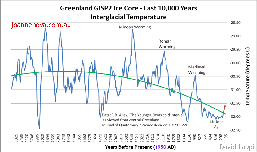
UPDATE: This graph shows the ice-core data up until 1855.

Think for a minute about how stupid this claim is that no single year, not one, in the last 125,000 years was warmer than the last 12 months. Cavemen are rolling in their graves.

It’s “virtually certain” said two journalists at Reuters. It was broken by 0.4 degrees!

Homo Sapiens have had satellite data for 44 years, which only leaves 124,956 years of extrapolation to guess at the rest. Not one journalist at the ABC, Sydney Morning Herald, CNN, or anywhere, asked the “scientists” — how would you know? Do tell us, professor, what exactly was the temperature from November 6,789 BC to October 6,788? And to a tenth of a degree, and globally. I heard it was hot?

Try to imagine what kind of miraculous science makes these headlines make sense?  Did the EU team find neolithic newspapers hidden in caves in Turkey? Could they reconstruct temperatures from 10,000 BC to 1978 to a tenth of a degree Celsius. And not just Turkish temperatures but ones in Timbuktu and Peru too? Those goat herders needed a satellite program.  Perhaps clay pots powered with goat dung?

ABC

It’s as if thousands of hotter Holocene years never existed

Studies all around the world show sea levels were as much as 1 – 2 meters higher 6,000 years ago, and have been falling for thousands of years. For example, studies on mangroves in Brazil show sea levels were about 2.7 meters higher in the mid-Holocene, and mangroves grew 34 kilometers further inland.  (Fontes et al 2017). How does that happen if the world was cooler then?

NoTricksZone lists sea level studies all over the world and CO2 Science lists other proxies. 6,000 years ago the world was so much warmer, the Sahara was lush green and wet. Even the sacred, revered ice cores from both Greenland and Antarctica show it was warmer. The deepest oceans around Indonesia were 2 degrees warmer 10,000 years ago. And 6,000 boreholes drilled around the world agree.

Glaciers in Europe were so much smaller, that as the world cooled and they grew, they swallowed up thousands of pieces of evidence. In the recent warming some 4,000 new tools, bridles, pieces of leather have melted out of Norwegian glaciers alone.

Many Pacific Island have only existed for three or four thousand years — emerging into the sunshine as sea levels fell from the Holocene peak.

This pattern of falling sea levels all over the world doesn’t fit the climate models. Instead of just admitting the models are wrong, researchers call their failure the “Holocene Temperature Conundrum”. We’re going to have to fight for the Holocene — the modelers want to erase it to solve the conundrum.

Shock news for alarmists, poor dears,
And sure to cause climate stress tears,
As 2023 beat,
All records of heat,
Kept for 125,000 years.

–Ruairi

REFERENCES

Alley, R. B. (2000) The Younger Dryas cold interval as viewed from central Greenland. Quat. Sci. Rev. 19, 213-226

Fontes et al (2017) The Impacts of the Middle Holocene High Sea-Level Stand and Climatic Changes on Mangroves of the Jucuruçu River, Southern Bahia – Northeastern Brazil, Radiocarbon , Volume 59 , Issue 1 , February 2017 , pp. 215 – 230.  DOI: https://doi.org/10.1017/RDC.2017.6

Huang, S. P., H. N. Pollack, and P.-Y. Shen (2008), A late Quaternary climate reconstruction based on borehole heat flux data, borehole temperature data, and the instrumental record, Geophys. Res. Lett., 35, L13703, doi:10.1029/2008GL034187   [PDF] Long blog discussion on boreholes.

Kench, P.S., Liang, C., Ford, M.R. et al. (2023) Reef islands have continually adjusted to environmental change over the past two millennia. Nat Commun 14, 508  doi.org/10.1038/s41467-023-36171-2

Lewis, S.E., et al., Post-glacial sea-level changes around the Australian margin: a review, Quaternary Science Reviews (2012), http://dx.doi.org/10.1016/j.quascirev.2012.09.006 [abstract] 

Hamish McGowan,Samuel Marx, Patrick Moss, Andrew Hammond (2012): Evidence of ENSO mega-drought triggered collapse of prehistory Aboriginal society in northwest Australia, Geophysical Research Letters, Vol 39, Issue 22.  DOI: 10.1029/2012GL053916 [Abstract]

Rehn, E. et al (2021) A late-Holocene multiproxy fire record from a tropical savanna, eastern Arnhem Land, Northern Territory, Australia [PDF]

Rosenthal, Y., Braddock K. Linsley, Delia W. Oppo (2013) Pacific Ocean Heat Content During the Past 10,000 Years, Science 1 November,Vol. 342 no. 6158 pp. 617-621  DOI: 10.1126/science.1240837 [Sciencemag.org ]

Yacoub et al., (2023), The African Holocene Humid Period in the Tibesti mountains (central Sahara, Chad): Climate reconstruction inferred from fossil diatoms and their oxygen isotope  composition

Kuper and Kropelin, (2006): Climate-controlled holocene occupation in the Sahara: motor of africa’s evolution. Science 313, 803e807. https://doi.org/10.1126/ science.1130989