A Demonstration: Low Correlations Do Not Necessarily Lead to Low Confidence in Data Regressions

In a recent post I used our new Urban Heat Island (UHI) warming estimates at individual U.S. GHCN stations having at least 120 years of data to demonstrate that the homogenized (adjusted) GHCN data still contain substantial UHI effects. Therefore, spurious warming from UHI effects is inflating reported U.S. warming trends.

From Roy Spencer, PhD

October 28th, 2024 by Roy W. Spencer, Ph. D.

In a recent post I used our new Urban Heat Island (UHI) warming estimates at individual U.S. GHCN stations having at least 120 years of data to demonstrate that the homogenized (adjusted) GHCN data still contain substantial UHI effects. Therefore, spurious warming from UHI effects is inflating reported U.S. warming trends.

The data plots I presented had considerable scatter, though, leading to concerns that there is large uncertainty in my quantitative estimates of how much UHI warming remains in the GHCN data. So, I updated that post to include additional statistics of the regressions.

A Simple Example: High Correlation, But Low Confidence In the Regression Slope

The following plot of a small amount of data I created shows what looks like a pretty strong linear relationship between 2 variables, with a regression explained variance of 82% (correlation coefficient of 0.91).

But because there are so few data points, there is large statistical uncertainty in the resulting diagnosed regression slope (21% uncertainty), as well as the regression intercept (which is diagnosed as 0.0, but with an uncertainty of +/- 0.94).

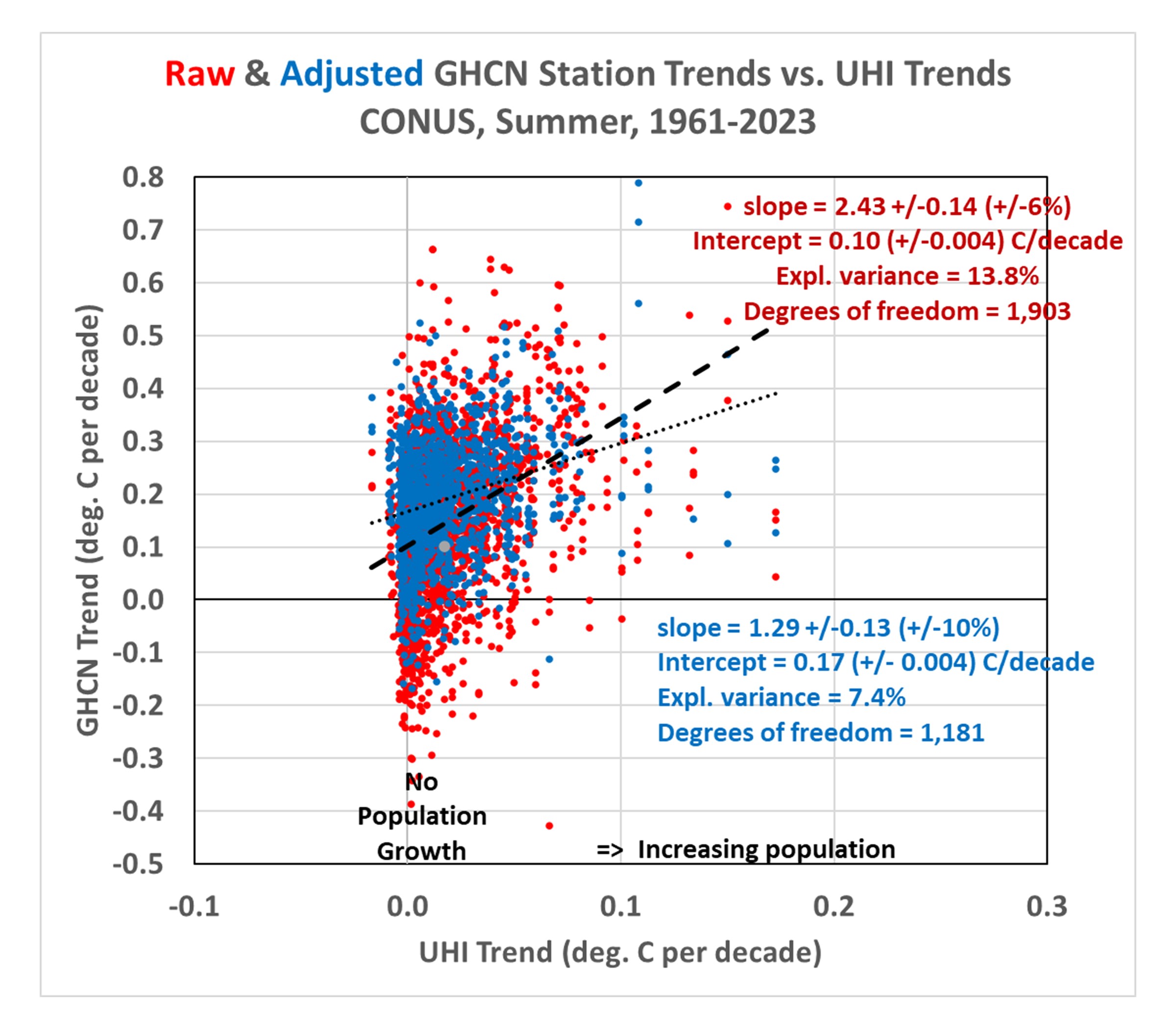
Now let’s look at the third data plot from my previous blog post, which demonstrated that there is UHI warming in not only the raw GHCN data, but in the homogenized data as well:

Importantly, even though the regression explained variances are rather low (17.5% for the raw data, 7.6% for the adjusted data), the confidence in the regression slopes is quite high (+/-5% for the raw GHCN regressions, and +/-10% for the homogenized GHCN regressions). Confidence is also high in the regression intercepts (+/-0.002 C/decade for the raw GHCN data, +/-0.003 C/decade for the homogenized GHCN data).

Compare these to the first plot above containing very few data points, which had a very high explained variance (82%) but a rather uncertain regression slope (+/- 21%).

The points I was making in my previous blog post depended upon both the regression slopes and the regression intercepts. The positive slopes demonstrated that the greater the population growth at GHCN stations, the greater the warming trend… not only in the raw data, but in the homogenized data as well. The regression intercepts of zero indicated that the data, taken as a whole, suggested zero warming trend (1895-2023) if the stations had not experienced population growth.

But it must be emphasized that these are all-station averages for the U.S., not area averages. It is “possible” that there has (by chance) actually been more climate warming at the locations where there has been more population growth. So it would be premature to claim there has been no warming trend in the U.S. after taking into account spurious UHI warming effects. I also showed that there has been warming if we look at more recent data (1961-2023).

But the main point of this post is to demonstrate that low correlations between two dataset variables do not necessarily mean low confidence in regression slopes (and intercepts). The confidence intervals also depend upon how much data are contained in the dataset.

A New Global Urban Heat Island Dataset: Global Grids of the Urban Heat Island Effect on Air Temperature, 1800-2023

Why is one neighborhood hotter than another? Chances are it is because it has fewer trees. Trees help cool neighborhoods down and reduce what’s called the “urban heat island effect”.

From Roy Spencer, PhD.

November 3rd, 2023 by Roy W. Spencer, Ph. D.

As a follow-on to our paper submitted on a new method for calculating the multi-station average urban heat island (UHI) effect on air temperature, I’ve extended that initial U.S.-based study of summertime UHI effects to global land areas in all seasons and produced a global gridded dataset, currently covering the period 1800 to 2023 (every 10 years from 1800 to 1950, then yearly after 1950).

It is based upon over 13 million station-pair measurements of inter-station differences in GHCN station temperatures and population density over the period 1880-2023. I’ve computed the average UHI warming as a function of population density in seven latitude bands and four seasons in each latitude band. “Temperature” here is based upon the GHCN dataset monthly Tavg near-surface air temperature data (the average of daily Tmax and Tmin). I used the “adjusted” (homogenized, not “raw”) GHCN data because the UHI effect (curiously) is usually stronger in the adjusted data.

Since UHI effects on air temperature are mostly at night, the results I get using Tavg will overestimate the UHI effect on daily high temperatures and underestimate the effect on daily low temperatures.

This then allows me to apply the GHCN-vs-population density relationships to global historical grids of population density (which extend back many centuries) for every month and every year since as early as I choose. The monthly resolution is meant to capture the seasonal effects on UHI (typically stronger in summer than winter). Since the population density dataset time resolution is every ten years (if I start in, say, 1800) and then it is yearly starting in 1950, I have produced the UHI dataset with the same yearly time resolution.

As an example of what one can do with the data, here is a global plot of the difference in July UHI warming between 1800 and 2023, where I have averaged the 1/12 deg spatial resolution data to 1/2 deg resolution for ease of plotting in Excel (I do not have a GIS system):

If I take the 100 locations with the largest amount of UHI warming between 1800 and 2023 and average their UHI temperatures together, I get the following:

Note that by 1800 there was 0.15 deg. C of average warming across these 100 cities since some of them are very old and already had large population densities by 1800. Also, these 100 “locations” are after averaging 1/12 deg. to 1/2 degree resolution, so each location is an average of 36 original resolution gridpoints. My point is that these are *large* heavily-urbanized locations, and the temperature signals would be stronger if I had used the 100 greatest UHI locations at original resolution.

Again, to summarize, these UHI estimates are not based upon temperature information specific to the year in question, but upon population density information for that year. The temperature information, which is spatial (differences between nearby stations), comes from global GHCN station data between 1880 and 2023. I then apply the GHCN-derived spatial relationships between population density and air temperature during 1880-2023 to those population density estimates in any year. The monthly time resolution is to capture the average seasonal variation in the UHI effect in the GHCN data (typically stronger in summer than winter); the population data does not have monthly time resolution.

In most latitude bands and seasons, the relationship is strongly nonlinear, so the UHI effect does not scale linearly with population density. The UHI effect increases rather rapidly with population above wilderness conditions, then much more slowly in urban conditions.

It must be remembered that these gridpoint estimates are based upon the average statistical relationships derived across thousands of stations in latitude bands; it is unknown how accurate they are for specific cities and towns. I don’t know yet how finely I can regionalize these regression-based estimates of the UHI effect, it requires a large number (many thousands) of station pairs to get good statistical signals. I can do the U.S. separately since it has so many stations, but I did not do that here. For now, we will see how the seven latitude bands work.

I’m making the dataset publicly available since there is too much data for me to investigate by myself. One could, for example, examine the growth over time of the UHI effect in specific metro regions, such as Houston, and compare that to NOAA’s actual temperature measurements in Houston, to get an estimate of how much of the reported warming trend is due to the UHI effect. But you would have to download my data files (which are rather large, about 117 MB for a single month and year, a total of 125 GB of data for all years and months). The location of the files is:

https://www.nsstc.uah.edu/public/roy.spencer

You will be able to identify them by name.

The format is ASCII grid and is exactly the same as the HYDE version 3.3 population density files (available here) I used (ArcGIS format). Each file has six header records, then a grid of real numbers with dimension 4320 x 2160 (longitude x latitude, at 1/12 deg. resolution).

Time for Willis to get to work.