Global warming, climate change, all these things are just a dream come true for politicians. I deal with evidence and not with frightening computer models because the seeker after truth does not put his faith in any consensus. The road to the truth is long and hard, but this is the road we must follow. People who describe the unprecedented comfort and ease of modern life as a climate disaster, in my opinion have no idea what a real problem is.
The Met Office is warning of the “strongest winds of the year” this week!
No doubt the BBC will exaggerate the storm and then blame it on global warming.
Well, I decided to take a shot at publishing my views on the cloud feedback response to increases in surface warming. I wrote it up and sent it for peer review to the Journal of Climate.
Well, I decided to take a shot at publishing my views on the cloud feedback response to increases in surface warming. I wrote it up and sent it for peer review to the Journal of Climate.
The reviewers said that it seemed like I was looking at changes in location, not changes over time. So I re-wrote it and sent it back in.
They wrote back and said ok, changes helped, and oh, by the way …
… it’ll cost you $1,546 to get it published.
I can assure you that I harnessed the awesome power that comes from splitting the infinitive. In a far-too-loud voice, I uttered various speculations regarding the ancestry, sexual habits, and personal hygiene of the Owners, Editors, and Reviewers. I fear I went so far as to encourage them to engage in auto-fornication … for all of which I’m truly sorry. It’s just what goes on in 2023, and I’m still not used to it.
So instead, I figured I’d start by publishing it here, and invite people to suggest changes, to point out inconsistencies, and to generally be some combination of Editors and Reviewers of the paper. Please be kind in your comments, I’m just a fool whose intentions are good.
With that as a prologue, here’s the current state of the paper.
Independent Climate Researcher, Occidental, California
Corresponding author: Willis Eschenbach
ABSTRACT
Cloud radiative response to a change in surface temperatures is a key component in accurately estimating future temperature changes. Changes in surface temperature lead to different cloud responses in different parts of the planet. However, the overall effect of these changes has been very poorly constrained. (Boucher 2013) Using data from satellite observations, I develop two independent methods to estimate how the clouds in different areas respond to a surface temperature increase. Both methods show a global net surface cloud radiative cooling effect. The size of the cooling obtained in this manner is a minimum value of total cloud cooling, because more cloud-related cooling occurs as a result of a temperature-related increase in thermally-driven tropical and extra-tropical thunderstorms which cool the surface in a variety of non-radiative ways. In addition, using theoretical arguments, I show that it is unlikely that the cloud response amplifies global warming.
1. Introduction
Clouds have a central role in modulating the global energy balance. They have long been recognized as being the major source of uncertainty in climate projections. Although a variety of evidence has been presented, a narrow constraint on how clouds respond to projected warming has remained elusive. Indeed, there is still no widespread agreement even on the sign of the cloud response to warming. Part of the challenge is that net cloud radiative effect involves cloud effects on both solar (shortwave [SW]) and terrestrial (longwave [LW]) radiative fluxes. (Ceppi et al. 2017, Gettleman and Sherwood 2016)
A most unusual yet generally unremarked feature of the climate system is its thermal stability. Here is the trough-to-peak temperature range over a 22-year period for each 1° latitude by 1° longitude gridcell.
Fig. 1. Maximum variations in monthly average temperature (trough to peak) during the period Mar 2000 – Feb 2022.
Here, we see temperature swings of over 30°C in the poles, 29°C over the land, 9°C over the oceans, and 14.8 °C for the globe as a whole. But despite those large intra-annual swings, after 12 months the temperature always returns to nearly the same value. Over the same Mar 2000 – Feb 2022 period, the CERES data reveals annual average global surface temperature changes of only about 0.5°C, which is only three percent of the intra-annual variation.
And as another example, over the entire 20th Century the temperature only increased by 0.8°C, which is a 0.3% temperature rise in 100 years.
Figure 2. Annual temperature ranges for the globe (red line) and monthly temperature ranges for parts of the globe. Red line shows range of 20th Century global average annual temperatures, around 0.3%.
As Figure 2 above shows, this surprising longer-term stability cannot be from thermal inertia, given the far larger monthly intra-annual swings. This overall steady-state condition argues strongly for the existence of natural thermoregulatory phenomena opposing any change in the overall steady-state temperature.
This is supported by Le Chatelier’s Principle. Le Chatelier enunciated a simple principle that governs systems that are in a steady-state condition. Le Chatelier’s principle asserts that a disturbance applied to a system at a steady state may drive the system away from its equilibrium state, but will invoke a countervailing influence that will counteract the effect of the disturbance. (Gorshkov et al. 1990) This principle strongly suggests that if the global average temperature changes, the clouds and other phenomena will act to counteract the temperature change, not to reinforce it.
The net cloud radiative effect (CRE) at the surface is composed of the clouds’ effect on two different types of radiation. The first is solar (shortwave) radiation, which is both reflected and absorbed by clouds. The second is thermal (longwave) radiation, which is both radiated and absorbed by clouds. The net surface CRE, which I’ll call “CRE” for simplicity, is the total of the two effects at the surface where we live. In other words, the CRE is the difference between downwelling radiation in clear-sky and cloudy-sky conditions. If the CRE is negative, it means clouds are cooling the surface.
In general, clouds cool the surface. Figure 3 shows the global variations in the CRE. In Fig. 3 we see that the clouds warm the poles and the deserts, and cool everywhere else.
Fig. 3. Surface cloud radiative effect, on a 1° latitude x 1° longitude basis.
The short-term change in surface CRE with temperature is easily calculated using the CERES data. Figure 4 shows that result.
Figure 4. Short-term trends in surface cloud radiative effect as a function of temperature. Trends are ordinary least squares linear regression slopes.
However, that doesn’t tell us what we need to know, which is how the clouds respond to a long-term change in surface temperature. Despite that, there are two ways that we can use observational data to measure that response.
Both of them depend on a simple idea—as a long-term average for each gridcell, over thousands of years, the temperature and the corresponding cloud radiative effect have reached a steady state condition. All of the various phenomena affecting the CRE, such as relative humidity, boundary-layer inversion strength, CAPE (Convective Available Potential Energy), oceanic subsidence and upwelling, and other factors now oscillate around long-term average values for each given gridcell. Thus, the average relationship between temperature and CRE for each gridcell represents the long-term steady-state relationship.
The first way to see what will happen if the surface temperature warms is a gridcell-based scatterplot of CRE and temperature.
Fig. 5. Scatterplot, 22-year averages of CRE versus surface temperature. Each dot is a 1° latitude by 1° longitude gridcell.
Despite this scatterplot including both land and ocean and covering from the tropics to both poles, there is a clear pattern. Looking from the left to the right in the scatterplot, the slope of the black/white line shows the direction and amount of change in the CRE as the temperature increases. There are four different zones.
The coldest zone encompasses the Antarctic and Greenland ice caps. Where the average monthly gridcell temperature is below -20°C, you are in one of those two locations. There, increasing temperatures lead to increasing cloud warming. This represents less than 4% of the planetary surface.
The next zone is from -20°C to 10-15°C. In this zone, increasing warming results in increasing cloud cooling. The third zone is from 10-15°C to about 25°C. In this zone, increasing temperature leads to increasing cloud warming.
Finally, in the warmest parts, increased surface warming leads to greatly increased cloud cooling. At its greatest, an increase of 1°C leads to up to 40 W/m2 of increased cloud cooling (reduction in downwelling surface radiation).
Now, this shows us the overall pattern of the relationship between temperature and CRE. It is extremely non-linear. But it is a general indication, with lots of scatter around the trend line. It also shows areas from all around the world combined.
What this method doesn’t show is either the detailed spatial pattern or the area-weighted global average response of the CRE to increasing temperature. For this I use a second method.
The second method looks only at the average values of the gridcells in the area immediately around each gridcell. Consider a gridcell in the ocean as an example. Nearby gridcells to the north, south, east, and west of that chosen gridcell will have different long-time average values for temperature and CRE. So we can determine the long-term effect by looking at the local relationship between average temperature and average CRE. For each gridcell, I have used a box that is 9° latitude by 9° longitude, centered on the chosen gridcell. This gives me 81 temperature values and a corresponding 81 CRE values. I do a linear regression of the 81 CRE values as a function of the 81 temperature values. The resulting slope shows the change in CRE corresponding to a 1° change in temperature. I’ve analyzed the land and the ocean separately, to avoid mixing different regimes. However, this seems to make little difference. The result is shown in the following Pacific- and Atlantic-centered graphics.
Fig. 6. Changes in surface cloud radiative effect per 1°C change in surface warming. The lower panel is the same as the upper but with an Atlantic-centered view. All values used in the calculation are the average of the full 22 years of the CERES record.
This shows two views, one Pacific and one Atlantic centered, of the detailed location and size of changes in CRE from 1°C surface warming. Globally, there is an area-averaged net cooling of -1.7 W/m2. The main cooling occurs over the ocean, with an area-averaged cooling of -2.4 W/m2. The land is the only area which is even slightly positive, with an area-averaged warming of +0.3 W/m2
These results are in good agreement with those of Ramanathan and Collins (Ramanathan, V., & Collins, W. (1991)), although the proposed mechanisms are different, and these results are for the planet while Ramanathan and Collins only looked at the Pacific Warm Pool.
3. Stability And Uncertainty
If this metric is indeed a measure of the long-term change in CRE with warming, it should change very little from year to year. The boxplot below shows 22 CRE feedback values for each geographical area listed in Figure 6, one for each year of the CERES record.
Figure 7. Boxplot, change in CRE from 1°C surface warming. Data for each of the 22 years in the CERES record.
As expected, there is very little variation in the results despite the shortness (one year) of each dataset. This indicates that even a 22-year average will give accurate values for the change in surface CRE per 1°C warming. As in Figure 6, the only large area that shows positive feedback is the land, and the feedback is quite small.
4. Data Details
I used monthly gridded Clouds and the Earth’s Radiant Energy System (CERES) Energy Balanced and Filled Edition 4.1 data (Loeb et al. 2018). The CERES record is quite stable (Loeb et al. 2016), which makes it an excellent record for this type of analysis. All of the CERES data used covers the 22-year period from March 2000 to February 2022.
For surface temperature, I have used the CERES surface upwelling longwave dataset, converted to temperature using the Stefan-Boltzmann equation. For verification of the calculated CERES surface temperature data, I have compared it with the results using the Berkeley Earth gridded land/ocean data record (Rohde and Hausfather 2020). The area-weighted average difference between the two is only 0.43°C. This difference is not surprising because the Berkeley Earth dataset is a combination of air temperature over land and sea surface temperature. On the other hand, the CERES data is surface temperature everywhere. Below is the same calculation shown in Figure 5 but using the Mar 2000 – Feb 2022 Berkeley Earth Data in place of CERES data for that same period. Note that there is very little difference between this and Figure 5 above which uses CERES data.
Figure 8. As in Figure 5, but using Berkeley Earth surface temperature data in place of CERES data.
5. Final Thoughts
As mentioned above, the cloud radiative effect is only one of the ways that the clouds affect the surface temperature. In addition, thunderstorms cool the surface by means of:
• Increased surface albedo over the ocean due to the white surface foam, spume (foam driven aloft by the wind), and spray. Increased cloud albedo due to the vertical extent of thunderstorm towers.
• A thunderstorm operates on the same refrigeration cycle as a household refrigerator or air conditioner. It evaporates a working fluid (in this case water) in the area to be cooled. It moves the resulting vapor to a separate physical location (the thunderstorm cloud base) where the working fluid is condensed and then returned to the area to be cooled, in the form of cold rain. This natural refrigeration-cycle heat engine greatly cools the surface quite independently of any radiation considerations.
• There is increased evaporative cooling due to the thunderstorm-generated winds at the base, as well as from the provision of dry air to the surface.
• A large thunderstorm typically generates on the order of 20,000 tonnes of rainfall over its existence. This means it is moving on the order of 40 terajoules of energy from the surface to high up in the troposphere. There, because it is above most greenhouse gases, it is much freer to radiate to space.
• Increased evaporation from the increase in surface area due to the creation of millions of spray droplets.
• Increased radiation to space due to the lack of water vapor in the dry descending air between the thunderstorms.
Tropical thermally driven thunderstorms increase with increasing temperatures. As a result, the cloud radiative cooling (CRE) is enhanced by increased thunderstorm production, and the CRE cooling estimates represent a minimum value.
Acknowledgments.
All of this work is my own. However, I owe immense thanks to all of the outstanding scientists who have preceded me. I have no conflicts of interest.
Boucher, O. et al., 2013: Clouds and aerosols, Climate Change 2013: The Physical Science Basis. Contribution of Working Group I to the Fifth Assessment Report of the Intergovernmental Panel on Climate Change (Cambridge University Press, Cambridge, UK, 2013), pp. 571–657.
Ceppi, P, F. Brient, M. D. Zelinka, D. L. Hartmann, 2017: Cloud feedback mechanisms and their representation in global climate models. Wiley Interdisc. Rev. : Clim. Change8, e465.
Gorshkov, V.G., Sherman, S.G. & Kondratyev, K.Y., 1990: The global carbon cycle change: Le Chatelier principle in the response of biota to changing CO2 concentration in the atmosphere. Il Nuovo Cimento C13, 801–816 https://doi.org/10.1007/BF02511997
Loeb, N. G. et al., 2018: Clouds and the Earth’s Radiant Energy System (CERES) Energy Balanced and Filled (EBAF) Top-of-Atmosphere (TOA) Edition-4.0 data product. J. Clim.31, 895–918.
Loeb, N., N. Manalo-Smith, W. Su, M. Shankar, S. Thomas, 2016: CERES top-of-atmosphere Earth radiation budget climate data record: Accounting for in-orbit changes in instrument calibration. Rem. Sens.8, 182.
Ramanathan, V., & Collins, W. (1991). Thermodynamic regulation of ocean warming by cirrus clouds deduced from observations of the 1987 El Niño. Nature, 351(6321), 27–32. doi:10.1038/351027a0 https://sci-hub.se/10.1038/351027a0
Rohde, R. A. and Hausfather, Z., 2020: The Berkeley Earth Land/Ocean Temperature Record, Earth Syst. Sci. Data, 12, 3469–3479, https://doi.org/10.5194/essd-12-3469-2020.
So, there it is. All comments, criticisms, and improvements gladly considered. This site provides one of the best peer-review processes on the planet.
Please remember that when you comment, you need to quote the exact words you are discussing. That way, we can all be clear about your subject.
Finally, a couple of requests.
First, I’d still like to get this sucker published. Does anyone know of a reasonably high-impact-factor journal that does NOT charge $1,546 to publish a paper?
And second, does anyone want to take this paper over and shepherd it through the review process? This method worked out very well for Craig Loehle and me. With some assistance from me, he rewrote parts of my post on extinctions entitled Where are the Corpses?, he arm-wrestled the journals, and we got it published as Historical bird and terrestrial mammal extinction rates and causes, with him as the Lead Author. So far, about 150 citations, with more each month.
Anyone interested? Any “publish or perish” folks out there not interested in perishing? Because I truly hate dealing with the journals …
My very best wishes to all, enjoy this marvelous world where we are given so little time.
Gridcells lacking sufficient sampling that month are left out of the averaging, and the uncertainty from such missing data is estimated. IMO that is more reasonable than inventing data to infill. And it seems that the Global Drifter Array displayed in the top image is providing more uniform coverage of the oceans than in the past.
The best context for understanding decadal temperature changes comes from the world’s sea surface temperatures (SST), for several reasons:
The ocean covers 71% of the globe and drives average temperatures;
SSTs have a constant water content, (unlike air temperatures), so give a better reading of heat content variations;
A major El Nino was the dominant climate feature in recent years.
HadSST is generally regarded as the best of the global SST data sets, and so the temperature story here comes from that source. Previously I used HadSST3 for these reports, but Hadley Centre has made HadSST4 the priority, and v.3 will no longer be updated. HadSST4 is the same as v.3, except that the older data from ship water intake was re-estimated to be generally lower temperatures than shown in v.3. The effect is that v.4 has lower average anomalies for the baseline period 1961-1990, thereby showing higher current anomalies than v.3. This analysis concerns more recent time periods and depends on very similar differentials as those from v.3 despite higher absolute anomaly values in v.4. More on what distinguishes HadSST3 and 4 from other SST products at the end. The user guide for HadSST4 is here.
The Current Context
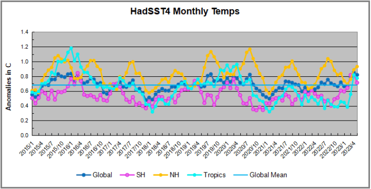
The chart below shows SST monthly anomalies as reported in HadSST4 starting in 2015 through May 2023. A global cooling pattern is seen clearly in the Tropics since its peak in 2016, joined by NH and SH cycling downward since 2016.
Note that in 2015-2016 the Tropics and SH peaked in between two summer NH spikes. That pattern repeated in 2019-2020 with a lesser Tropics peak and SH bump, but with higher NH spikes. By end of 2020, cooler SSTs in all regions took the Global anomaly well below the mean for this period. In 2021 the summer NH summer spike was joined by warming in the Tropics but offset by a drop in SH SSTs, which raised the Global anomaly slightly over the mean.
Then in 2022, another strong NH summer spike peaked in August, but this time both the Tropic and SH were countervailing, resulting in only slight Global warming, later receding to the mean. Oct./Nov. temps dropped in NH and the Tropics took the Global anomaly below the average for this period. After an uptick in December, temps in January 2023 dropped everywhere, strongest in NH, with the Global anomaly further below the mean since 2015.
Now comes El Nino as shown by the upward spike in the Tropics since January, the anomaly nearly doubling from 0.45C to 0.83C. SH stayed the same as March, but NH also increased 0.13, resulting in a Global anomaly of 0.85C. However, in May 2023, both the Tropics and SH temps dropped down, reducing the Global anomaly to 0.82C dispite an upward bump in NH.
A longer view of SSTs
The graph above is noisy, but the density is needed to see the seasonal patterns in the oceanic fluctuations. Previous posts focused on the rise and fall of the last El Nino starting in 2015. This post adds a longer view, encompassing the significant 1998 El Nino and since. The color schemes are retained for Global, Tropics, NH and SH anomalies. Despite the longer time frame, I have kept the monthly data (rather than yearly averages) because of interesting shifts between January and July.1995 is a reasonable (ENSO neutral) starting point prior to the first El Nino.
The sharp Tropical rise peaking in 1998 is dominant in the record, starting Jan. ’97 to pull up SSTs uniformly before returning to the same level Jan. ’99. There were strong cool periods before and after the 1998 El Nino event. Then SSTs in all regions returned to the mean in 2001-2.
SSTS fluctuate around the mean until 2007, when another, smaller ENSO event occurs. There is cooling 2007-8, a lower peak warming in 2009-10, following by cooling in 2011-12. Again SSTs are average 2013-14.
Now a different pattern appears. The Tropics cooled sharply to Jan 11, then rise steadily for 4 years to Jan 15, at which point the most recent major El Nino takes off. But this time in contrast to ’97-’99, the Northern Hemisphere produces peaks every summer pulling up the Global average. In fact, these NH peaks appear every July starting in 2003, growing stronger to produce 3 massive highs in 2014, 15 and 16. NH July 2017 was only slightly lower, and a fifth NH peak still lower in Sept. 2018.
The highest summer NH peaks came in 2019 and 2020, only this time the Tropics and SH were offsetting rather adding to the warming. (Note: these are high anomalies on top of the highest absolute temps in the NH.) Since 2014 SH has played a moderating role, offsetting the NH warming pulses. After September 2020 temps dropped off down until February 2021. In 2021-22 there were again summer NH spikes, but in 2022 moderated first by cooling Tropics and SH SSTs, then in October to January 2023 by deeper cooling in NH and Tropics.
Now in 2023 the Tropics flip from below to above average, and NH starts building up for a summer peak comparable to previous years. In May warming in the Tropics and SH abated, while NH showed a typical upward bump.
What to make of all this? The patterns suggest that in addition to El Ninos in the Pacific driving the Tropic SSTs, something else is going on in the NH. The obvious culprit is the North Atlantic, since I have seen this sort of pulsing before. After reading some papers by David Dilley, I confirmed his observation of Atlantic pulses into the Arctic every 8 to 10 years.
Contemporary AMO Observations
Through January 2023 I depended on the Kaplan AMO Index (not smoothed, not detrended) for N. Atlantic observations. But it is no longer being updated, and NOAA says they don’t know its future. So I find only the Hadsst AMO dataset has data through April. It differs from Kaplan, which reported average absolute temps measured in N. Atlantic. “Hadsst AMO follows Trenberth and Shea (2006) proposal to use the NA region EQ-60°N, 0°-80°W and subtract the global rise of SST 60°S-60°N to obtain a measure of the internal variability, arguing that the effect of external forcing on the North Atlantic should be similar to the effect on the other oceans.” So the values represent differences between the N. Atlantic and the Global ocean.
The chart above confirms what Kaplan also showed. As August is the hottest month for the N. Atlantic, its varibility, high and low, drives the annual results for this basin. Note also the peaks in 2010, lows after 2014, and a rise in 2021. An annual chart below is informative:
Note the difference between blue/green years, beige/brown, and purple/red years. 2010, 2021, 2022 all peaked strongly in August or September. 1998 and 2007 were mildly warm. 2016 and 2018 were matching or cooler than the global average. 2023 is starting out slightly warm.
Summary
The oceans are driving the warming this century. SSTs took a step up with the 1998 El Nino and have stayed there with help from the North Atlantic, and more recently the Pacific northern “Blob.” The ocean surfaces are releasing a lot of energy, warming the air, but eventually will have a cooling effect. The decline after 1937 was rapid by comparison, so one wonders: How long can the oceans keep this up?
Footnote: Why Rely on HadSST4
HadSST is distinguished from other SST products because HadCRU (Hadley Climatic Research Unit) does not engage in SST interpolation, i.e. infilling estimated anomalies into grid cells lacking sufficient sampling in a given month. From reading the documentation and from queries to Met Office, this is their procedure.
HadSST4 imports data from gridcells containing ocean, excluding land cells. From past records, they have calculated daily and monthly average readings for each grid cell for the period 1961 to 1990. Those temperatures form the baseline from which anomalies are calculated.
In a given month, each gridcell with sufficient sampling is averaged for the month and then the baseline value for that cell and that month is subtracted, resulting in the monthly anomaly for that cell. All cells with monthly anomalies are averaged to produce global, hemispheric and tropical anomalies for the month, based on the cells in those locations. For example, Tropics averages include ocean grid cells lying between latitudes 20N and 20S.
Gridcells lacking sufficient sampling that month are left out of the averaging, and the uncertainty from such missing data is estimated. IMO that is more reasonable than inventing data to infill. And it seems that the Global Drifter Array displayed in the top image is providing more uniform coverage of the oceans than in the past.
USS Pearl Harbor deploys Global Drifter Buoys in Pacific Ocean
Get ready. The El Nino is going to be weaponized and it gives people that argue natural causes for warming a golden opportunity to show the other side of the issue.
The coming El Nino provides a great chance to expose that simply buying that CO2 is the most significant climate control knob is folly.
This would cut the supposed scientific support out from ESG and WEF policies further exposing their agenda which is plainly anti-American Prosperity and freedom.
The CFSV2 has some members ( blue) with a Super Nino Developing. The blue members are the most recent run the red past runs.
forecast at this time in 2015
While Super Ninos have occurred. there is simply no analog to the Atlantic and how warm it is. Take for instance the forecast for ASO 2015. vs now
The huge difference is in the Atlantic. ( outlined in the hurricane impact forecast) So CAGW people push increases in Greenhouse gases for the reason, which you will see in the chart later is highly improbable.
But this is going to have major implications for the weather for a year or 2 down the road and in the climate situation. In addition, we know what is going to happen with the global temperature response. another step up is coming. This will provide people arguing the natural side of Global Warming an opportunity to counter the onslaught coming from Agenda driven man-made climate people, on the cause. To argue Enso events like this, which VISIBILY LEAD TO STEP UPS IN GLOBAL TEMPERATURES DUE TO IMMENSE WATER VAPOR INPUT AND THE CORRELATION IT HAS IN THE COLDEST DRIEST AREAS
are due to man-made influences borders on the absurd. Something has to be warming the oceans, and it is not the US input that has resulted in .0000125 of the atmosphere being co2 ( total co2 is .0042). Basically, the Green new deal is sacrificing the US’s future prosperity on an altar that is worshipping a false God in the name of a Marxist global agenda.
Look at the energy content of the system
Atmospheric warming is the RESULT of larger-scale warming, not the cause of it. So again what is warming the ocean? It is not the air. Co2 does have properties to warm the air, but not to the extent that is attributed. And again, a nation with a small and decreasing contribution of this should not be committing what amounts to societal suicide because of it
Personally, I am excited about this, I hope people on my side of the issue, that believe this is natural, get ready and get out in front. That is the problem. For some reason, people that are in the media or whatever, refuse to get out in front of the predictable reactions from the leftist. And then you are left to fight sound bite for sound bite with an overwhelming amount of people in power that refuse to even look.
For whatever reason the oceans are warming, it can not be explained by CO2 input But the warming of the air can be explained by the warming of the ocean. I have pointed out that if we quantified water vapor increase in grams/kg, then correlated it to the saturation mixing ratios with temperatures, you would likely see the lion’s share of where it is warming more and how much has to do with that. So why do we just look at CO2? Makes no sense.
I am already out front with my hypothesis, which is being widely trashed from both sides, and that is fine. ( the idea is that this increase is negligible and I have no proof. The reason I have no proof is because of the amazing lack of research on this matter. But they have no proof it is not. So given the oceanic effect on temperature, why are we not putting time and effort into that, instead of the relentless almost mindless drumbeat of how horrible it is despite life never being better?) Latest Seismic activity charts show a sudden drop-off
If this were to persist then the test of my idea is lurking, oceans after the super Nino would cool, and the air should follow to some extent after a small lag period
But remember TSI has been on the increase and is linked directly to WV. ( Dr. Willie Soon has been the leader in this aspect)
Seismic activity vs global temp
Both of these certainly correlate better than CO2
Get ready. The El Nino is going to be weaponized and it gives people that argue natural causes for warming a golden opportunity to show the other side of the issue. In fact, whether I am on to something or not, at the least, the other people with explanations will have a chance to show the multitude of counters to a tunnel-visioned nonscience approach (the argument is settled nothing else to see here) to explaining what we see. It would not be so bad, except it has been co-opted and turned into one of a multitude of half-truths designed to destroy our way of life, you pick the topic, and the link is there.
WeatherBell has been the pioneer in trying to alert the public as to where these storms are going to go. My long-standing idea is that numbers can be a red herring and even not valuable, as the biggest problem is where the storms wind up impacting. This year could be a classic example. It will feature a potentially top-10 El Niño versus a warm Atlantic. How much oxygen the El Niño can suck out of the room is not a normal slam dunk.
I am confident of a below average season for Central America and the Caribbean. A lot of the African wave energy may be left in the form of storms to the east of 50°W that recurve. The fear is a feeding frenzy near our coasts with in-close development. As long as the Atlantic is warm that will always be a concern, but an El Niño is no cause for relaxation.
We have taken the lead on creating a Power and Impact scale which is meant to quantify the overall power of storms better. This is done for two reasons. Firstly, the user will know more about the storm’s nature. Secondly, it helps quantify a storm for historical comparisons. Donna, Charley, and Ian were all double-hitting Category 4s from Florida to the Carolinas, but in terms of Power and Impact, Donna was greater than Ian and much greater than Charley (as far as size). For a more detailed explanation, please visit https://www.weatherbell.com/power-and-impact-scale.
Forecast Discussion
With the state of the oceans, we are in no-mans-land, awash in a sea of warmth. The widespread warmth distorts effects by spreading them out over a greater area. That will make this season a unique El Niño. El Niño is a part of this year’s forecast and a big one, but in this case, its average effects may be mitigated. The Euro’s tropical forecast is bizarre. It is above average in the Atlantic and East Pacific, but below normal in the West Pacific. The first and last forecast runs are completely opposite of what has happened in El Niños as strong as the model is forecasting.
Typically an El Niño is a slam-dunk-below-normal-activity forecast, by simply taking the blend of those events. There are two problems with that. First, the statistical models are not nearly as warm as the Euro and other dynamical models. They of course are based on statistics that incorporate years not as warm.
Obviously, a weaker El Niño means a different input. The aborted El Niño of 2017 is a prime example. Then again in 2017, the dynamical models were not off to the races:
So now let’s assume the models are right. The SSTs in those years looked like this:
However, the Atlantic is much warmer this year:
I will discuss the implications below with comparisons for Sea Level Pressure and precipitation.
Now compare that to the active years in the Atlantic Basin:
So while we are going to use the analogs, we understand their use is limited this time around.
As I mentioned, the Euro forecast is strange. It has the West Pacific below normal and the East Pacific above, which is fine. However, it also has the Atlantic above normal. A look at the analog years reveals how bold that is.
Those years would give us a bit under 8 storms per year, 3-4 hurricanes, and 1 major hurricane per year. The average ACE Index is near 50! Those are way, way under what we have at the top. The Euro is forecasting 15 total storms and 6.5 hurricanes, with an ACE index of 120. I read that as a lot of little storms.
Now let’s look at the precipitation patterns in the strong El Niño seasons:
Here is the Euro for the heart of the hurricane season (ASO):
Active seasons:
We see striking similarities in the southwestern Caribbean, but the Atlantic Basin is shown to be a bit wetter than the average El Niño year. Certainly, it is closer to that than the active years.
Sea Level Presure in stong El Niños:
The Euro:
Active years:
The trademark low pressure to the west of South America is there. This means stronger easterlies and wind sheer over the eastern Pacific. However, pressures over the Atlantic are shown to be near normal, which means the easterlies won’t be as strong there. We don’t get to where we are in the active years in the Atlantic Basin because of low pressure over the Gulf of Mexico and the Tropical Atlantic.
The 500 mb in El Niños:
The Euro:
Active seasons:
The Euro forecast is an antilog to the active seasons, though is not as far to the north. What is very strange is the positives all through Asia. That is the opposite of El Niño years.
In addition, a look at the CFSv2 clearly shows a tendency for less shear around the Gulf of Mexico and Southeast, especially in the front part of the season. That means an early season storm or two can really get things started (1957 Audrey and 1972 Agnes for example).
JJA:
JAS:
ASO:
An active season like 2020 certainly has the opposite:
This year we do have less to the north of the “red zone” that stands out so clearly in non-active years. Keep in mind this is the most active season on record, but the point is around the Gulf of Mexico and Florida there was less hostility.
West Pacific forecast
We have had a 3-year period of very low typhoon activity (and landfalling activity). That should come to an end. The Euro likes the landfalls but with less than average ACE, which is baffling to me. For East Asian interests, the trend should be over. For climate interests, if you don’t get an ACE bounceback to well above in this pattern, then I think the screaming and yelling about the tropics has got to stop. It becomes absurd. ACE Index is not increasing, for one, but the shutdown of the West Pacific over the last 3 years with no major above normal activity to counter it with this kind of El Niño would really be a nail in that coffin. I do think we will have some major landfalling typhoons this year, though, more so than in the last 3 years.
The Verdict
I hope I have laid out the parameters here in a way you can understand what we are looking at. I have written about the weakening of the Hadley Cell and dropping 400 mb humidities over the Main Development Regions of the world, a distortion of the pattern due to major warming away from the Tropics likely has a role in that. This year for the Atlantic Basin we will have an El Niño that I think can get to +1.5°C (the CFSv2, Canadian, and Euro are all at +2°C) but it is surrounded by global SSTs that are so warm that we have not seen anything like it, let alone an El Niño year. So modeling is trying to handle inputs that it may not be able to.
My take is that the Atlantic is warm enough that the farther away from the Main Development Region the more the chance for development relative to normal. That means the U.S. is in an area close to it.
Joe Bastardi is a pioneer in extreme weather and long-range forecasting.
He is the author of “The Climate Chronicles: Inconvenient Revelations You Won’t Hear From Al Gore — and Others” which you can purchase at the CFACT bookstore.
His new book The Weaponization of Weather in the Phony Climate war can be found here. phonyclimatewar.com




You must be logged in to post a comment.