Global warming, climate change, all these things are just a dream come true for politicians. I deal with evidence and not with frightening computer models because the seeker after truth does not put his faith in any consensus. The road to the truth is long and hard, but this is the road we must follow. People who describe the unprecedented comfort and ease of modern life as a climate disaster, in my opinion have no idea what a real problem is.
In eastern Uganda, a mother can spend two hours a day gathering firewood to cook her family’s meals. Incredibly, 85% of Ugandan households still cook with wood and 13% depend on charcoal. Smoky indoor fires are estimated to cause thousands of premature deaths in the country every year, while clean-burning liquefied petroleum gas (LPG) reaches fewer than one home in a hundred. A billion sub-Saharan Africans are without clean fuel for cooking.
Standing between life and death is the European Investment Bank (EIB), the lending arm of the European Union that ended financing for fossil-fuel projects at the end of 2021. The World Bank runs a similar playbook. Last December, it issued a $200 million Clean Cooking Outcome Bond whose Ghana projects cover 245,000 electric cookers and 170,000 improved biomass stoves but not one LPG cylinder.
The body count Brussels ignores
According to the World Health Organization (WHO), household air pollution killed an estimated 2.9 million people in 2021. Soot from cooking fires has been blamed for nearly half of all deaths from lower respiratory infections in young children. Africa bears the heaviest share with an estimated 815,000 premature deaths a year.
WHO lists LPG and natural gas among the clean cooking fuels it wants expanded. The International Energy Agency (IEA) expects gas to supply more than 60% of the African households that gain access to clean cooking through 2040. Its roadmap calls for spending about $2 billion a year to introduce clean cooking to 80 million people annually.
So, the world’s leading health agency calls LPG clean. The world’s leading energy agency calls it the main pathway out of smoke. Which guidelines, then, are the EIB and World Bank following?
Did a single European family wait for a foreign lender’s blessing before trading coal stoves for gas burners in the last century? Of course not. Gas lifted Europe’s women out of soot-filled kitchens, and they have never looked back.
Before the invasion of Ukraine, Russia supplied about 45% of the EU’s gas and LNG imports. Brussels condemned Moscow and imposed sanctions. Yet the bloc imported a record 106 million metric tons of LNG in 2025, with Russia ranking as its second-largest supplier at about 14%.
The buying did not slow even as the ban approaches. In the first half of 2026, EU buyers took a record 9.97 million metric tons from Russia’s Yamal LNG plant, worth more than $6 billion and 16% above the year before, stocking up ahead of the full prohibition that begins at the beginning of 2027.
The double standard extends to Europe’s closest partners. Norway, bound to the EU through the European Economic Area, places no ceiling on petroleum development. Oslo awarded 57 offshore production licenses in January, after issuing 53 in 2025 and 62 in 2024. Each license grants rights to explore, drill, and extract. Across six years, Norway has handed out 333 of them. You will search in vain for an EIB statement condemning any of it.
A bloc that pays a geopolitical adversary for gas has no moral standing to deny an African widow a cooking cylinder.
Patricia Nanteza, Africa coordinator at WePlanet, told the Monitor that LPG is the most accessible clean option families have in the near term and that lifting the ban would free more households from biomass. When climate campaigners themselves plead for financing of gas, the ban has lost its last defense.
The EIB and World Bank policies that protect their climate scorecards while African women devote half their lives carrying water and children are lost to early death. That trade carries no scientific, moral, or economic justification.
Vijay Jayaraj is a Science and Research Associate at theCO2 Coalition, Fairfax, Virginia. He holds an M.S. in environmental sciences from the University of East Anglia and a postgraduate degree in energy management from Robert Gordon University, both in the U.K., and a bachelor’s in engineering from Anna University, India. He served as a research associate with the Changing Oceans Research Unit at University of British Columbia, Canada.
The Natufian culture was a late Epipalaeolithic archaeological culture of the Levant (West Asia), dating roughly from about 15,000- 11,500 years before present (cal BP), or approximately 13,000- 9,500 BCE.
The Natufian culture (roughly 15,000- 11,500 cal BP) developed and changed against a backdrop of major late Pleistocene climate oscillations in the Levant. Climate strongly influenced settlement patterns, mobility, resource use, and ultimately the path toward agriculture, though the exact mechanisms and degree of impact remain debated.
AI generated by Grok
The Natufian culture was a late Epipalaeolithic archaeological culture of the Levant (West Asia), dating roughly from about 15,000- 11,500 years before present (cal BP), or approximately 13,000- 9,500 BCE.
It is named after Wadi en- Natuf (near Shuqba Cave in the West Bank), where British archaeologist Dorothy Garrod first identified it in 1928 during excavations.
Key Characteristics
The Natufians are especially notable as one of the earliest known societies to develop sedentary or semi-sedentary lifestyles while still relying primarily on hunting and gathering, before full agriculture. They are widely viewed as a transitional culture that set the stage for the Neolithic Revolution and the world’s earliest farming villages.
Chronology: Commonly divided into Early Natufian (roughly 15,000/13,000- 13,000/11,500 cal BP) and Late Natufian (ending around 11,500 cal BP). The Late phase overlapped with the cooler, drier Younger Dryas climatic period.
Geography: Centered in the Levant, modern- day Israel, the Palestinian territories, Jordan, Lebanon, and parts of Syria (with some extension toward the Euphrates). Key zones included the Mediterranean woodland hills, the Jordan Valley, and adjacent steppe areas.
Subsistence: Intensive hunting (especially gazelle) and gathering of wild plants, particularly cereals (wild barley, wheat, rye), nuts, legumes, and other seeds. They used flint sickle blades (often with characteristic sheen from plant cutting) set in bone or wood handles, plus abundant ground- stone tools (mortars, pestles, grinding slabs) for processing plants. Evidence includes early bread- like remains (e.g., at Shubayqa 1 in Jordan, ~14,400 years ago) and possible fermented cereal residues (e.g., at Raqefet Cave). Some sites show possible low-level cultivation or intensive management of wild cereals, though full domestication came later. Dogs appear as the earliest domesticates.
Settlement and Architecture: Semi- sedentary base camps and hamlets with circular or oval semi-subterranean dwellings featuring stone foundations, hearths, postholes, and sometimes storage features. Larger open- air sites (such as ʿAin Mallaha (Eynan), el-Wad, and Wadi Hammeh 27) show repeated, long- term occupation. Caves and rock shelters were also used.
Technology and Material Culture: Geometric microliths (especially lunates) are diagnostic. Rich bone- tool assemblages (including sickles), personal ornaments (shell beads, especially dentalium), and art (carved bone and stone figures, abstract designs, and rare figurative pieces such as the “Ain Sakhri Lovers”). Long- distance exchange of materials occurred.
Burial Practices and Social Life: Cemeteries within or near settlements, often with personal ornaments. Some evidence of secondary burial, skull treatment, and possible social differentiation. Ritual and symbolic behavior intensified, including possible feasting.
Significance and Major Sites
The Natufian marks a shift toward greater sedentism, intensified plant use, more complex social organization, and ritual investment. These changes occurred among the last purely foraging societies in the region before farming communities appeared. Successors include the Harifian (in the south) and the Pre-Pottery Neolithic (PPNA).
Important sites include:
Shuqba Cave (type site)
ʿAin Mallaha (Eynan)
el-Wad, Hayonim, and Raqefet Cave (Mount Carmel area)
Beidha
Tell Abu Hureyra
Wadi Hammeh 27 (an Early Natufian open- air settlement near Pella, Jordan, with substantial architecture and recent finds of foundational burials)
In short, the Natufians represent a pivotal “threshold” culture in human prehistory, bridging mobile Paleolithic foragers and the settled agricultural societies of the Neolithic Near East.
A map of the Levant with Natufian regions across present-day Israel, the Palestinian territories, Jordan, Sinai, and a long arm extending into Lebanon and Syria
Wadi Hammeh 27 is indeed a significant Late Epipalaeolithic archaeological site near Pella (Tabaqat Fahl) in the Jordan Valley, Jordan. It preserves remains of a substantial Early Natufian settlement dating roughly to 14,500- 14,000 years ago (cal BP).
Key points that match and expand on the description:
It belongs to the Early Natufian phase of the Natufian culture (part of the broader Epipalaeolithic sequence in the Levant).
Excavations (notably by Phillip Edwards and others) uncovered evidence of a relatively large, semi-sedentary community, including multiple structures, hearths, and dense concentrations of cultural material.
Finds typically include ground- stone tools (mortars, pestles), microliths, bone tools, ornaments, and abundant faunal and botanical remains that illuminate early steps toward sedentism and intensive plant use in the region.
The site sits in the Wadi al- Hammeh drainage and is one of the better- preserved Early Natufian open- air settlements known from Jordan.
Wadi Hammeh 27 is firmly dated to the Early Natufian period. The settlement was occupied for a relatively short span of roughly 500 years.
Key dating summary
Overall range: Approximately 12,500- 12,000 cal BC (or about 14,500- 14,000 years ago / cal BP). This places it firmly in the Early Natufian, before the onset of the Younger Dryas.
Radiocarbon evidence (main AMS dates from carbonized seeds and other organic material):
Classic dates from Phase 1 (uppermost occupation):
OxA-393: 11,920 ± 150 BP
OxA-507: 11,950 ± 160 BP
OxA-394: 12,200 ± 160 BP These calibrate to roughly 12,000- 11,500 cal BC (with broader ranges possible).
Newer AMS dates from Phase 4 (foundational layers and burials, published in recent work):
Around 12,290- 12,438 BP, calibrating to approximately 12,700- 12,200 cal BC. These support an initial foundation of the burial ground and earliest occupation near 12,500 BCE.
Stratigraphic phases
The site has four main occupation phases (from lowest to highest):
Phase 4 (basal): Foundational burials established on travertine/bedrock (~12,500 BCE). Houses were later built directly over these graves. No further burials occurred after this phase.
Phases 3- 2: Intermediate architectural phases with continued occupation and commemorative features over the original graves.
Phase 1 (uppermost): Final substantial occupation with large oval stone dwellings, ending around 12,000 cal BC.
The entire sequence represents continuous or repeated use of the same location as a substantial “base camp” for several centuries, after which the site was abandoned. Sedimentation continued in the wadi after abandonment (e.g., Melanopsis shell date of ~11,100 BP).
In short, Wadi Hammeh 27 is one of the best-dated and earliest large open- air Early Natufian settlements in the southern Levant, spanning the later part of the Bølling– Allerød warming phase.
Wadi Hammeh 27 (Early Natufian, ~12,500- 12,000 cal BC / ~14,500- 14,000 cal BP) was occupied entirely during the later part of the Bølling- Allerød interstadial, a relatively warm and moist climatic phase that followed the Last Glacial Maximum. The site was abandoned before the full onset of the colder Younger Dryas.
Timeline (calibrated years)
Period
Approximate Dates
Climate Conditions
Relation to Wadi Hammeh 27
Late Glacial Maximum & early deglaciation
Before ~14,700 cal BP
Cold and relatively dry
Pre- occupation
Bølling- Allerød interstadial (warming)
~14,700- 12,900 cal BP
Warmer and wetter than preceding glacial conditions; expanded Mediterranean woodlands, higher lake levels in the region, increased plant productivity (wild cereals, oak, pistachio, etc.)
Full occupation of the site (~12,500–12,000 cal BC). Favorable conditions supported semi- sedentary base-camp life with substantial architecture, intensive plant harvesting (wild barley, etc.), and rich resource base. Local environment was moister than today, possibly with a nearby freshwater lake or high-water table.
Onset of Younger Dryas
~12,900- 12,700 cal BP
Rapid cooling begins (globally colder; in the Levant often cooler, with debated degree of drying)
Site occupation ends around or just before this transition (~12,000 cal BC). No clear evidence of occupation continuing into the full Younger Dryas.
Younger Dryas
~12,900- 11,500 cal BP
Cooler (and in many reconstructions drier or with altered seasonality)
Post- abandonment. The site was no longer occupied.
Early Holocene warming
After ~11,500 cal BP
Rapid return to warmer and wetter conditions
Long after the site was abandoned
Local environmental notes for the site
During occupation the surrounding landscape was more humid than the modern arid Jordan Valley, supporting oak woodland elements, wild cereals (especially barley), pistachios, lentils, and other edible plants.
The site sat in a spring- fed wadi system. Some researchers suggest it may have overlooked a temporary freshwater lake (sometimes called “Damya Lake”) or experienced elevated water levels related to the late stages of Lake Lisan.
After abandonment (~12,000 cal BC), regional lake levels continued to change, and the wadi eventually incised as base levels dropped following the final drying of Lake Lisan around 11,000 BP.
In short, Wadi Hammeh 27 flourished under the relatively benign, resource -rich conditions of the late Bølling- Allerød warming and was deserted before the climatic stress of the Younger Dryas fully set in. This places it among the classic Early Natufian settlements that benefited from the post- glacial climatic amelioration.
The Natufian culture (roughly 15,000- 11,500 cal BP) developed and changed against a backdrop of major late Pleistocene climate oscillations in the Levant. Climate strongly influenced settlement patterns, mobility, resource use, and ultimately the path toward agriculture, though the exact mechanisms and degree of impact remain debated.
Climatic Context
The Natufian spanned the transition from the end of the Last Glacial Maximum into the early Holocene, encompassing:
Bølling- Allerød interstadial (roughly 14,700- 12,900 cal BP): A warmer and generally wetter phase that supported expanded Mediterranean woodlands (oak- pistachio forests) and abundant wild plant resources, including cereals. This period largely coincides with the Early Natufian.
Younger Dryas (YD) (roughly 12,900- 11,500 cal BP): A sharp, globally recognized return to colder conditions lasting about 1,200- 1,500 years (somewhat longer or differently expressed in the Levant). The Late Natufian largely overlaps with this event.
Onset of the Holocene: Rapid warming and wetter conditions after ~11,500 cal BP, coinciding with the end of the Natufian and the rise of the Pre- Pottery Neolithic A (PPNA).
Paleoclimate reconstructions (from pollen, speleothems, lake levels, charcoal, and isotopic data from gazelle teeth) show the Early Natufian flourished under relatively favorable conditions: higher precipitation (sometimes exceeding modern levels in places) and temperatures closer to or slightly below present- day values, fostering productive woodlands and cereal stands.
During the Younger Dryas, conditions became cooler (especially during the growing season). Traditional models emphasized strong drying and contraction of woodlands, but more recent isotopic evidence from gazelle tooth enamel indicates cooling without significant aridification in the southern Levant, water availability for plants remained similar or even higher than in the preceding phase. Seasonal contrasts may have been reduced, with potential effects on cereal productivity and harvest timing.
Climate Impacts on Natufian Culture
Early Natufian (warmer and wetter phase):
Favorable climate supported greater sedentism. Larger base camps and hamlets with durable stone architecture (e.g., Wadi Hammeh 27, ʿAin Mallaha) appeared, along with intensified plant processing (sickles, ground stone tools) and denser occupation. Resource abundance in Mediterranean woodlands and the Jordan Valley enabled semi- permanent settlements.
Late Natufian (Younger Dryas):
Cooler conditions are linked to shifts toward greater residential mobility, smaller or more dispersed sites in some areas, changes in burial practices, and possible intensification or broadening of diets (more small game, birds, or alternative plants). Some groups may have moved toward more climatically buffered zones such as the Jordan Valley, where wild cereals remained more productive. Site distributions show expansion into certain steppe or desert- margin areas.
Not all researchers see the YD as a severe crisis that forced agriculture. Some argue Late Natufians successfully adapted through increased mobility and demographic adjustments rather than immediate cultivation. Continuity of occupation exists in many regions, and the Levant may have served as a refugium.
Link to the origins of agriculture:
A long- standing hypothesis holds that YD stress on wild cereal stands (reduced productivity or reliability due to cooler temperatures) pressured sedentary populations, who had become dependent on these resources, to begin more intensive management or early cultivation. This is thought to have contributed to the emergence of farming in the subsequent PPNA after the climate improved. Other views emphasize that Natufians remained successful foragers throughout the YD and that agriculture arose more gradually under improving early Holocene conditions, or through a combination of social, demographic, and environmental factors.
Summary of Key Dynamics
Climate acted as an important but not sole driver.
The warm and wet Bølling- Allerød facilitated the Early Natufian florescence of sedentism and plant intensification.
The cooler Younger Dryas prompted adaptive responses (greater mobility in some areas, possible settlement shifts) without fully collapsing the culture.
The rapid post- YD warming then coincided with the transition to Neolithic farming villages. Regional variation was significant, Mediterranean core areas, the Jordan Valley, and peripheral steppes responded differently, and ongoing research continues to refine local climate reconstructions and their precise cultural correlations.
A recent post at far-left news outlet Mother Jones, “There’s a Powerful, Hidden Force Behind Migration: Climate Change,” claims that climate change is a powerful driver of mass migration from the third world. This is false. The migrants themselves who were interviewed only bring up weather at all when pressed to do so, economic factors are the usually cited reasons for both illegal and legal attempts at migration to western countries. Extreme weather is not at all new to the regions discussed.
A recent post at far-left news outlet Mother Jones, “There’s a Powerful, Hidden Force Behind Migration: Climate Change,” claims that climate change is a powerful driver of mass migration from the third world. This is false. The migrants themselves who were interviewed only bring up weather at all when pressed to do so, economic factors are the usually cited reasons for both illegal and legal attempts at migration to western countries. Extreme weather is not at all new to the regions discussed.
The author claims that recent mass migration to Spain and other countries from places like Morocco is secretly being spurred on by climate change, and suggests that media does not often discuss that factor. This is immediately absurd, of course, because the mainstream media often cites climate change as a driver of both legal and illegal immigration. Climate Realism has recently debunked such claims regarding migrants from Somalia, here, for instance.
Undermining the initial claim of the headline and introduction, the author admits “[t]hat is not to say that the effects of climate change caused tens of thousands of people to risk their lives by attempting to swim to Ceuta. Economic forces were much more urgent motivators for Mohamed to leave his home.”
The migrant interviewed by Mother Jones says that the reason he is trying to leave Morocco is because of limited job opportunities. He does not mention climate change at all. But the author goes on to insist “after another summer of extreme temperatures and wildfires in the northern and southeastern provinces in Morocco, severe flash flooding and landslides in rural communities throughout the High Atlas Mountains, and the culmination of a seven-year drought after a winter of heavy rainfall across the country, climate change also may be an underlying factor in creating the economic crisis forcing so many to leave their homes.”
This is completely backwards. The reason these severe weather events have such a large impact on Morocco and other poorer countries is because they are weak economically in the first place, making it difficult or impossible for communities to invest in weather hardened infrastructure. The cited extreme weather events are not new to the region, and happen all around the world regardless of climate change.
Flash flooding is a feature of desert environments, once dry seasons are over. Likewise, drought for that matter is an obvious feature of the desert, especially lengthy droughts, which the author admits recently came to an end. Alternating periods of extended drought and deluge are the norm for Morocco in particular. The southeastern Morocco desert has recently seen dry lakebeds refill with water, when they have been mostly empty for a long time due to the recent drought period. Those lakebeds would not be there in the first place if they did not sometimes fill. Trying to claim that these natural patterns are evidence of climate change is nonsense.
As for the wildfires, again wildfire is not new to the region, and data from the joint NASA and European Space Agency joint project Copernicus show that there is no trend towards worsening wildfires in Morocco, neither in area burned nor number of fires. (See figure below)
Despite 2022 seeing a record bad fire year, 2024 was a record low for wildfires in Morocco since records begin in 2002 according to Copernicus data. Mother Jones is not interested in that, only the high years. Good scientists would not claim that 2024 represented a trend towards the elimination of wildfire, and likewise 2022 is not indicative of a trend towards climate catastrophe.
The Mother Jones post goes on to make the dubious claim that “North Africa and the Middle East are warming faster than the rest of the world, and Morocco’s agricultural sector—the cornerstone of the country’s economy—is particularly vulnerable to climate impacts like soil degradation and depleted groundwater.”
Soil degradation and depleted groundwater are resource management impacts, not climate impacts. For example, the same claim was made about depleted water resources in Nigeria, but population growth stressing the water supply around Lake Chad and other countries upriver building dams were the real cause. Natural drought under those conditions is bound to make things worse.
The most notable part of this article is the straightforward dismissal of the actual complaints of the migrants themselves, in order to push the climate claim. The so-called experts that the author interviews insist basically that the migrants don’t know what they are talking about, that climate change is the real background issue, instead of things like political corruption and violence making economies unstable in the region and hindering development.
The data do not show anything unprecedented happening with the weather, but it is clear that Mother Jones is not interested in facts.
Researchers at the Swedish University of Agricultural Sciences (SLU) developed a method using “bomb carbon” (elevated radiocarbon- 14 from 1960s atmospheric nuclear tests, preserved in tree rings) in wood shavings to track how stable biochar is when added to soil.
AI generated by Grok
Researchers at the Swedish University of Agricultural Sciences (SLU) developed a method using “bomb carbon” (elevated radiocarbon- 14 from 1960s atmospheric nuclear tests, preserved in tree rings) in wood shavings to track how stable biochar is when added to soil.
Biochar is a charcoal- like material produced by heating biomass (here, wood) in low- oxygen conditions (pyrolysis). It is of interest for improving soil properties and as a potential long-t erm carbon sink to help mitigate climate change, with global estimates suggesting it could sequester carbon equivalent to roughly 6- 16% of annual anthropogenic CO₂ emissions. A key uncertainty has been how quickly biochar mineralizes (breaks down into CO₂) in soil versus remaining stable for decades or centuries, and how to distinguish its contribution from native soil organic matter.
The method
Atmospheric nuclear testing in the 1950s- 1960s roughly doubled atmospheric ¹⁴C levels, peaking around the mid-1960s. Tree rings from 1964-1967 therefore contain elevated “bomb” ¹⁴C. SLU researchers selected mature Norway spruce and Scots pine trunks from a Swedish clear- cut, identified the relevant rings, and used a professional woodturner to carefully remove outer wood and collect the thin, high-¹⁴C layers as shavings. These were pyrolyzed into biochar (tested at highest treatment temperatures of ~400°C and 650°C).
The resulting biochar had enough ¹⁴C enrichment (on average ~61.7 percent modern carbon higher than bulk soil organic matter in one report) to serve as a natural tracer. In a one-year laboratory incubation, they mixed it into soil (at 2% by dry mass), trapped emitted CO₂, and measured its ¹⁴C signature via accelerator mass spectrometry. This allowed them to quantify the share of CO₂ coming from the biochar versus the soil.
Key findings
CO₂ from biochar- amended soil showed up to about 10% higher ¹⁴C than controls, confirming a small but measurable contribution from the biochar.
Roughly 0.35% of the added biochar carbon converted to CO₂ over one year.
This implies high stability: at least half of the buried biochar is projected to remain in the soil after ~200 years (under the study conditions).
The method works with mature wood feedstock that resembles commercial biochars, offers higher precision than some natural- abundance ¹³C approaches, and avoids the need for expensive artificial isotopic labeling.
The work was published in Radiocarbon (Li et al., 2026: “Bomb ¹⁴C for tracing biochar mineralization in soil”). It was funded in part by Sweden’s Bio+ program (Swedish Energy Agency). Follow- up research is planned to examine biochar stability under climate- change scenarios in collaboration with researchers in Germany.
This approach provides a practical way to study biochar persistence, its interactions with soil organic matter, and its viability for carbon sequestration without relying solely on short- term incubations or complex lab labeling.
To obtain wood formed during the years 1964–1967, the researchers engaged professional woodturner and wood artist Åke Landström from Glanshammar. Credit: Harald Cederlund
Bomb 14C for tracing biochar mineralization in soil
This is the open- access research article “Bomb ¹⁴C for tracing biochar mineralization in soil” by Haichao Li, Harald Cederlund, Elias S. Azzi, Cecilia Sundberg, and Erik Karltun (Swedish University of Agricultural Sciences), published online 23 September 2026 in Radiocarbon (Volume 68, Issue 5, pp. 1146- 1154).
It is freely available under a Creative Commons Attribution (CC- BY) licence.
Core contribution
The authors introduce and validate a practical isotopic- tracing method that uses naturally elevated “bomb” radiocarbon (¹⁴C) preserved in tree rings formed during the atmospheric nuclear- test peak (1964- 1967). Biochar made from this wood carries a clear ¹⁴C signature that can be distinguished from soil organic matter (SOM), allowing precise quantification of how much of the CO₂ released from soil comes from the biochar itself.
Methods (summary)
Mature Norway spruce and Scots pine trunks (≥70 years old) were collected from a clear- cut near Uppsala, Sweden.
Annual rings from 1964- 1967 were identified by counting and carefully isolated by professional woodturning (producing shavings).
Biochar was produced by pyrolysis under N₂ at highest treatment temperatures of 400 °C (BC400) and 650 °C (BC650). The feedstock with the highest ¹⁴C enrichment (~172.9 pMC) was selected.
Biochars were acid- washed to remove carbonates, ground (<2 mm), and mixed into a loamy- sand agricultural soil (Cambisol, 1.4 % SOC) at a 2 % (w/w) application rate.
Soils were incubated for 365 days at ~20.7 °C and 60 % water- holding capacity. Emitted CO₂ was trapped in NaOH and analysed for total C and ¹⁴C (AMS) at multiple time points.
An isotope-mixing model calculated the biochar- derived fraction of respired CO₂. Priming effects on native SOC were also quantified.
Key results
Biochar was on average 61.7 pMC higher in ¹⁴C than bulk soil organic matter, providing a clear tracer signal.
¹⁴CO₂ from biochar- amended soils was consistently and significantly higher than from controls (p < 0.0001).
Early in the incubation (first 2 weeks) 8.3- 11.4 % of mineralized CO₂- C came from biochar; later this fell to 2.3- 7.5 %.
After one year, only 0.32 ± 0.02 % (BC400) and 0.35 ± 0.01 % (BC650) of the added biochar carbon had been mineralized. The two pyrolysis temperatures did not differ significantly.
BC650 produced a measurable negative priming effect on native soil organic carbon (–129 ± 20 mg CO₂-C kg⁻¹, or ~14.8 % relative to the control); BC400 showed essentially none.
Advantages claimed over other isotopic approaches
Higher precision than the natural- abundance ¹³C (C₃/C₄) method for detecting small biochar contributions.
Works with mature wood feedstock that closely resembles commercial biochars (unlike many laboratory pulse- labelled materials derived from young seedlings).
Relatively low cost and does not require specialised isotope-labelling facilities.
Uniform ¹⁴C enrichment because the trees grew continuously under elevated atmospheric ¹⁴C.
Conclusions
The bomb-¹⁴C method is shown to be effective for quantifying biochar mineralisation and its interactions with soil organic matter. It opens practical possibilities for longer- term studies of biochar persistence and carbon-sequestration potential under realistic conditions.
The paper includes supplementary material with additional figures on priming and sensitivity analyses. Funding came in part from the Swedish Energy Agency’s Bio+ programme.
Log with younger wood turned away. The wood with the highest content of ‘bomb carbon’ is found in the growth rings between the red circles. Credit: Harald Cederlund
Journal:Radiocarbon (Volume 68, Issue 5, pp. 1146–1154)
Improving our understanding of biochar carbon (C) stability in soil is crucial given its potential for soil C sequestration. However, challenges with isotopic labeling of biochar restrict our ability to determine its fate in soil. Atmospheric nuclear bomb tests in the 1960s resulted in a 14C spike in tree rings, providing an opportunity to address this challenge. Here, we present a method that utilizes the elevated levels of 14C in wood from tree rings formed between 1964 and 1967 as a tracer to determine the proportion of biochar C in mineralized soil. Biochar was produced using wood from the 14C enriched tree rings as feedstock and thereafter used in a mineralization experiment capturing the emitted CO2. We demonstrate that the bomb 14C-enrichment in the biochar is high enough to differentiate between CO2 originating from either biochar or soil organic matter mineralization. The method can be used to address questions on biochar persistence, its interactions with soil organic matter and research that is needed to explore the potential to use biochar for C sequestration in soils.
“AI” is too broad to regulate as one thing. None of those everyday AI systems are actually what people are arguing about when they call for regulation, so just saying “AI” is way off the mark.
Because we “literally do not know what we are talking about,” policies passed in panic could be highly destructive.
Protest against ai technology robot holding no ai sign amidst determined crowd in urban setting
Debating policies in a rational manner requires a clear specification of the thing under consideration for regulation. The AI debate has nothing like that.
The AI debate does not even name the thing under discussion, as it is certainly not AI per se. Not being able to name the thing you are talking about is impossibly vague when it comes to policy making.
The field of AI is over 70 years old, and it has spawned a lot of different technologies, which are not part of the policy issue, so simply talking about AI is way off the mark.
Chess-playing machines that can beat grandmasters are an early example. There are now lots of AI game systems. My favorite is the blackjack program that saved me a lot of money by showing me I was no good at that gambling game.
In the late 1980s, expert systems became prominent. More recently, we got things like automated customer service systems and GPS routing systems. Now we have automated cars and military fighter drones. None of these are part of the AI policy discussion, nor are countless other AI systems in everyday use.
The AI issue mostly started with chatbots, which are typically called large language models (LLMs), so these are a good starting point. But there are lots of LLMs, some of which seem pretty harmless. The little AI summary that comes with each Google search, for example.
Plus, there are other AI systems besides LLMs that may be of concern. Examples include generative AI, diffusion models, and the interesting-sounding generative adversarial networks.
Then, too, there are AI agents that use models to perform instructed tasks. Concern about agents recently arose when a bunch started working together without being instructed to do so. We have no idea how many such systems exist.
The first thing a policy, law, or regulation must do is make clear who or what is covered and not covered. This is why regulations often have lengthy definition sections. They often create their own language in order to clearly specify the rules they state.
The AI policy debate has no such specificity. The things under discussion are not even named in many cases. As a Chinese philosopher friend of mine used to say, “We are talking in a vacuum.” Specifically, a cognitive vacuum which lacks needed substance.
Absent a clear specification of what we mean, any rules passed are likely to simply create destructive paralysis and confusion.
For example, people are talking about a pause in AI development. Which AI development? For that matter, what counts as AI development? This is another empty concept.
Let’s take Google. Last year, its R&D spending was over $60 billion. How much is AI related such that it would be paused? Some of it is labeled as AI development, but a lot of it is directly related to developments that have AI aspects, such as AI data centers.
It all depends on how AI is defined for the purposes of the pause, and there is not a shadow of a definition at this point. The potential for destructive confusion is immense. AI-related industry could run to trillions of dollars.
At the same time, there is much talk about an AI race, especially between America and China. I have yet to see this race defined or explained. Race to do what? What does winning look like? How are we doing?
It is not like there is going to be just one AI system, rendering all others obsolete. AI is a huge industrial domain with a vast number of diverse products. What then is this race?
The whole AI policy debate borders on being incoherent because we literally do not know what we are talking about. This is very dangerous because incoherent policies passed in panic can be highly destructive.
Researchers at Arizona State University (led by Bruce Rittmann of the Biodesign Swette Center for Environmental Biotechnology), with collaborators from Rice University, Tongji University, the National University of Singapore, and Nanjing University, developed a catalytic “hunter- killer” membrane that both captures and chemically destroys PFAS (“forever chemicals”) rather than just concentrating them.
The membrane technology developed by Arizona State University researchers (led by Bruce Rittmann) and international collaborators is a catalytic hollow-fiber membrane system designed to both capture and chemically destroy PFAS (“forever chemicals”).
AI generated by Grok
Researchers at Arizona State University (led by Bruce Rittmann of the Biodesign Swette Center for Environmental Biotechnology), with collaborators from Rice University, Tongji University, the National University of Singapore, and Nanjing University, developed a catalytic “hunter- killer” membrane that both captures and chemically destroys PFAS (“forever chemicals”) rather than just concentrating them.
PFAS are synthetic compounds used in nonstick coatings, waterproof fabrics, firefighting foams, and many other products. Their extreme persistence comes from very strong carbon- fluorine bonds (often called the strongest in organic chemistry), which shield the carbon backbone and resist breakdown by conventional biological or chemical processes. Standard treatments (activated carbon, ion exchange, membrane filtration) remove them from water but leave concentrated waste that still needs disposal or destruction.
How the technology works
Hollow- fiber membranes are coated on the outside with palladium nanoparticles.
Pressurized hydrogen gas is fed through the interior of the fibers and diffuses outward to the palladium catalyst.
The palladium splits H₂ into highly reactive hydrogen atoms.
PFAS molecules from the surrounding water adsorb onto the same palladium surface.
At the catalyst surface, the reactive hydrogen attacks and breaks the C- F bonds (hydrodefluorination), stripping fluorine and converting the persistent molecules into less harmful components.
This “inside- out” hydrogen delivery is a key design feature: the membrane both concentrates the pollutants at the reactive surface and supplies the activated hydrogen needed to dismantle them.
Performance results
In a continuous 58- day laboratory test treating a mixture of six regulated- priority PFAS compounds, the system removed more than 90% of each compound and stripped away about 83% of the total fluorine, confirming actual chemical destruction rather than simple filtration. Rittmann described the mechanism as essentially universal across the six compounds tested.
Practical considerations and next steps
Palladium is expensive (roughly $50,000 per kilogram), so reducing catalyst loading is a major research priority. The approach is envisioned as a complement to existing concentration methods: conventional filtration would first shrink large volumes of contaminated water into a smaller waste stream that the catalytic membrane then destroys. Hybrid systems pairing the palladium catalyst with pollutant- degrading bacteria are also under development.
This builds on earlier ASU work with membrane biofilm reactors (MBfR) and membrane catalyst- film reactors (MCfR) that combine catalytic defluorination with microbial degradation. While further engineering is needed for full- scale water treatment, the results demonstrate a promising route to permanently break down these persistent pollutants.
A palladium-coated membrane uses hydrogen to help break down PFAS “forever chemicals.” Credit: Jason Drees
The membrane technology developed by Arizona State University researchers (led by Bruce Rittmann) and international collaborators is a catalytic hollow- fiber membrane system designed to both capture and chemically destroy PFAS (“forever chemicals”).
Core design
Hollow- fiber membranes: Tiny tubular (“straw-like”) gas- transfer membranes.
Palladium nanoparticle coating: A thin layer of palladium nanoparticles is deposited on the outside of the fibers. Palladium acts as a catalyst.
Hydrogen delivery: Pressurized hydrogen gas (H₂) is fed through the inside of the hollow fibers. It diffuses outward through the membrane wall to the palladium layer.
How it works (“hunter- killer” mechanism)
Hydrogen reaches the palladium surface and is split into highly reactive atomic hydrogen.
PFAS molecules in the surrounding water adsorb onto the same palladium surface.
At the catalyst surface the reactive hydrogen attacks the strong carbon- fluorine bonds (hydrodefluorination), stripping fluorine atoms from the PFAS molecules.
This breaks the “forever” chemical structure, converting the compounds into less persistent (and ultimately more biodegradable) products.
The inside- out hydrogen supply is a key innovation: the membrane simultaneously concentrates the pollutants at the reactive surface and delivers the activated hydrogen needed to destroy them.
Performance
In a continuous 58- day laboratory trial treating a mixture of six regulated- priority PFAS compounds, the system:
Removed >90% of each individual PFAS.
Stripped ~83% of the total fluorine (confirming actual chemical destruction rather than mere capture).
Context and next steps
This builds on earlier ASU membrane technologies (Membrane Biofilm Reactor- MBfR and Membrane Catalyst- film Reactor- MCfR). Hybrid versions that combine the palladium catalyst with pollutant-degrading bacteria are also under development.
Main practical hurdle: Palladium is expensive (~$50,000/kg), so reducing catalyst loading is a priority. The technology is expected to work best as a polishing/destruction step after conventional concentration methods (e.g., activated carbon or ion exchange) have first reduced the volume of contaminated water.
The research was published in the Proceedings of the National Academy of Sciences in October 2026.
Catalytic reactive-hydrogen membranes for rapid capture and hydrodefluorination of six PFAS of regulatory concern
This peer- reviewed paper reports the development and continuous testing of a hydrogen- based Membrane Catalyst -film Reactor (MCfR) for simultaneous capture and destruction of PFAS (“forever chemicals”).
It reports the development and continuous testing of a hydrogen- based Membrane Catalyst- film Reactor (MCfR) for simultaneous capture and destruction of PFAS (“forever chemicals”).
Key elements of the paper (from published summaries)
Lead institution & author: Arizona State University’s Biodesign Swette Center for Environmental Biotechnology; senior/corresponding author Bruce E. Rittmann.
Collaborators: Researchers from Rice University (Texas), Tongji University (China), National University of Singapore, and Nanjing University (China).
Technology: Hollow- fiber gas- transfer membranes coated on the exterior with palladium (Pd) nanoparticles. Hydrogen gas is supplied from the lumen (inside) of the fibers, diffuses outward, and is activated on the Pd surface. PFAS molecules adsorb to the same surface, enabling catalytic hydrodefluorination (breaking of strong C- F bonds by reactive hydrogen).
Results: In a continuous 58- day operation treating a mixture of six regulatory-priority PFAS compounds, the system achieved >90% removal of each compound and ~83% overall fluorine removal (defluorination), confirming chemical destruction rather than simple separation.
Significance: Demonstrates a “universal” catalytic mechanism effective across the tested PFAS. The approach is positioned to treat concentrated waste streams after conventional separation processes. Palladium cost and catalyst loading reduction are noted as practical challenges; hybrid Pd–microbial systems are also referenced as ongoing work.
This builds on the group’s earlier Membrane Catalyst- film Reactor (MCfR) platform for catalytic reduction of oxidized contaminants using efficient H₂ delivery.
Direct full- text access may require institutional login or purchase via the PNAS site, as the open-page retrieval was restricted. The news coverage from ASU- affiliated and science outlets (e.g., Eurasia Review, Interesting Engineering, Bioengineer.org) provides consistent, detailed summaries of the findings.
Per- and polyfluoroalkyl substances (PFAS) persist in aquatic environments due to their ultrastable C–F bonds and poor susceptibility to conventional treatment. Here, we report an H2-based catalytic-film membrane that enables PFAS destruction in ambient conditions by generating highly reactive surface (Hads*) and subsurface hydrogen (Hsub*), the latter stored as β-phase palladium hydride (β-PdHx). Solid-state analyses evidenced β-PdHx formation and related lattice expansion with elevated H2 chemical potential, revealing a structural mechanism that links hydrogen storage to catalytic defluorination. Mechanistically, the two hydrogen species play complementary roles: Hads*-rich Pd0 surface enabled PFAS capture through parallel adsorption to maximize interfacial contact with active H, whereas sustained Hsub* supplied the energetic driving force for stepwise hydrodefluorination consistent with sequential C–F scission. As a result, across six PFAS of regulatory concern—PFOA, PFOS, PFNA, PFHxS, PFBS, and GenX—the catalytic membrane converted all contaminants toward fully defluorinated products. Long-chain PFAS were removed and defluorinated more rapidly than short-chain analogs, while GenX showed greater recalcitrance due to its ether linkage, weaker adsorption, and higher average C–F bond dissociation energy; nonetheless, GenX still exhibited removal and defluorination, with the production of 2-propoxypropanoic acid. The system also enabled continuous coremoval of all six PFAS in ambient conditions, with up to 96% removal and 83% defluorination over 58 d. These findings provide a mechanistic framework for how active hydrogen is generated, stored, and deployed in catalytic membranes, and identify engineered H2-catalytic membranes as a promising low-energy technology for destructive PFAS treatment.
Guterres’ hysteria rests on three weak legs: a worst-case scenario that its own authors have now abandoned, a “pre-industrial” baseline drawn from one of the coldest centuries in 2,000 years, and almost total silence about warm periods that preceded multi-megawatt power plants and SUVs by hundreds and thousands of years.
For more than a decade, projections of flooded coasts and failed harvests were driven by RCP8.5 and its successor SSP5-8.5. The article says they assumed 12 billion people by 2100 and a near tenfold rise in coal use.
Three years ago, U.N. Secretary-General António Guterres told reporters that “the era of global boiling has arrived.” In September he repeated the alarm. Launching the U.N.’s first report on temperature “overshoot,” he declared, “Humanity is speeding past the limit to avoid climate catastrophe.”
Guterres’ hysteria rests on three weak legs: a worst-case scenario that its own authors have now abandoned, a “pre-industrial” baseline drawn from one of the coldest centuries in 2,000 years, and almost total silence about warm periods that preceded multi-megawatt power plants and SUVs by hundreds and thousands of years.
Start with the scenario. For more than a decade, a computer-based hypothetical case called RCP8.5 and its successor SSP5-8.5 drove the most frightening projections of flooded coasts and failed harvests. They assumed a world of 12 billion people by 2100 and a near tenfold rise in coal use, a future predicted by no energy market.
This April, the modelers who design scenarios for the next generation of climate simulations conceded the point. Their projections of high levels of carbon dioxide emissions (CO2) had become “implausible,” and their update showed about 0.9 degrees Celsius less warming by century’s end. In August, the U.S. government proposed amending its Fifth National Climate Assessment so that results based on earlier projections can no longer be labeled “expected” or “business-as-usual.”
Now examine the yardstick. Every headline about crossing a 1.5-degree threshold measures warming from an 1850-1900 average. Those decades sit at the end of the Little Ice Age, an era when “livestock died, harvests failed, and humans suffered.” Choose the bottom of a cold trough as zero and every degree of recovery reads like a fever.
The most serious misdirection is what the panic merchants leave out. Earth’s climate swung widely long before anyone burned coal. A 2013 reconstruction in Science found that in comparison to today, intermediate Pacific waters were 2.1 degrees warmer during the Holocene Thermal Maximum 8,000 years ago and about 0.65 degrees warmer during the Medieval Warm Period 1,000 years ago. Tree rings from Finnish Lapland show that earlier estimates of warmth were too low.
Alaska’s retreating Mendenhall Glacier has exposed upright spruce and hemlock stumps more than 1,000 years old, a forest that grew where ice later advanced. At the Schnidejoch pass, more than 8,000 feet up in the Swiss Alps, melting ice has yielded more than 300 artifacts left by Neolithic, Bronze Age, Roman, and medieval travelers who crossed the mountains when the route was open. Certainly, temperatures warmer than today had prevailed.
Forecasts of heat-induced doom overlook the benefits of today’s elevated levels of atmospheric carbon dioxide. A NASA-led study found that a quarter to half of Earth’s vegetated land grew significantly greener over a 35-year period, with CO2 fertilization explaining 70% of the gain. The year after the world supposedly crossed the threshold of 1.5 degrees, the world’s farmers brought in a record cereal harvest, according to FAO data.
Humans have always faced weather hazards. Floods, droughts, storms, heat waves, crop failures, and changing rainfall existed before the industrial age. They will exist whether a theoretical global average temperature is 1.8 degrees Celsius or 2.8 degrees above an arbitrary baseline. The question is not whether risk exists, but how people respond to it.
And this is where having energy supplies that are reliable, affordable, and abundant helps people manage nature’s challenges. Economies that become more prosperous, maintain reliable systems, strengthen infrastructure, and reduce vulnerabilities will do more to protect human beings from climatic hazards even if they do not satisfy U.N. emission targets.
The future trajectory of CO2 emissions will be influenced overwhelmingly by the growth of energy demand in Asia and Latin America. There can be no justification for telling developing societies there that they must remain poor so that wealthy nations can preserve a global temperature target that has no scientific basis.
The U.N. fabricated an emergency, using a scenario its own modelers now call implausible, employing a baseline estimated rather than observed, and erasing warm eras that ancient farmers, traders, and travelers lived through. That is not science, but stagecraft performed for power and self-enrichment as it made the rest of the world poorer.
Originally published at Town Hall, October 19th, 2026.
Vijay Jayaraj is a Science and Research Associate at theCO2 Coalition, Fairfax, Virginia. He holds an M.S. in environmental sciences from the University of East Anglia and a postgraduate degree in energy management from Robert Gordon University, both in the U.K., and a bachelor’s in engineering from Anna University, India. He served as a research associate with the Changing Oceans Research Unit at University of British Columbia, Canada.
A recent study (published in Science Advances) indicates that Earth’s metallic core has been leaking primordial hydrogen, along with helium- 3 and certain tungsten isotopes, into the mantle for much of the planet’s 4.5- billion- year history.
Hydrogen moves from Earth’s core to the mantle primarily through limited chemical exchange and diffusion (or related transport) across the core, mantle boundary (CMB), rather than large- scale bulk flow.
Tungsten isotope anomalies, particularly involving the isotope ¹⁸²W, are important geochemical tracers used to study early Earth differentiation and possible ongoing exchange between Earth’s core and mantle.
AI generated by Grok
A recent study (published in Science Advances) indicates that Earth’s metallic core has been leaking primordial hydrogen, along with helium- 3 and certain tungsten isotopes, into the mantle for much of the planet’s 4.5- billion- year history.
Researchers from the University of Science and Technology of China used machine- learning- boosted path- integral simulations to model the quantum behavior of light atoms (especially hydrogen) under the extreme pressures and temperatures of the deep Earth. They focused on deuterium- to-hydrogen (D/H) ratios and related isotope signatures.
Key points from the work and related coverage:
Magma- ocean crystallization alone cannot explain the extremely low (deuterium- depleted) hydrogen isotope signatures seen in some ocean- island basalts (OIBs), such as those from Baffin Island and Iceland. These lavas rise from near the core, mantle boundary and carry chemical “messengers” from depth.
Primordial (solar- nebula) hydrogen stored in the core preferentially partitions as the lighter isotope. As it migrates upward, it lowers the mantle’s local D/H ratio. Supporting evidence comes from high ³He/⁴He ratios (primordial helium- 3 mixed with radiogenic helium- 4) and tungsten- isotope anomalies that also point to core material.
The hydrogen does not appear as free liquid water in the core; once it enters the oxygen- rich mantle it can form water bound in minerals. Over geologic time this exchange has dynamically altered the deep mantle’s composition rather than leaving purely “relic” signatures from early differentiation.
This builds on earlier experimental work (e.g., 2026 Nature Communications studies) showing the core itself may contain the equivalent of roughly 9- 45 oceans’ worth of hydrogen (0.07- 0.36 wt %), acquired mainly during Earth’s accretion rather than solely from later cometary delivery. Some of that reservoir appears to have been leaking upward for billions of years.
The quantities involved are tiny on human timescales, but the long-term chemical exchange helps explain observed isotope anomalies in surface rocks and improves models of Earth’s volatile budget, mantle dynamics, and early water origins. The findings reinforce that the core- mantle boundary is not a perfect chemical barrier.
Schematic model for the origin of isotopic anomalies in ocean island basalts. Credit: Science Advances (2026). DOI: 10.1126/sciadv.aei4756
Hydrogen moves from Earth’s core to the mantle primarily through limited chemical exchange and diffusion (or related transport) across the core, mantle boundary (CMB), rather than large- scale bulk flow.
This process has operated over billions of years and is supported by isotope evidence (especially low δD values) in ocean- island basalts that rise from near the CMB.
Key mechanisms
Chemical reactions and exchange at the CMB Subducted hydrous minerals can dehydrate in the lowermost mantle, releasing hydrogen (or water). This reacts with iron- silicon alloys from the outer core, forming phases such as iron hydride (FeHₓ) or related compounds. The reaction enables bidirectional exchange: hydrogen can enter the mantle side while silicon (as SiO₂) may move the other way. A hydrogen- rich, lower- density layer can form near the top of the outer core or accumulate at the base of the mantle (potentially contributing to ultralow- velocity zones). Because of its low density, some of this hydrogen- rich material migrates into the lowermost mantle.
Diffusion (including isotopic diffusion) Atomic diffusion of hydrogen across the CMB is a viable transfer route. Hydrogen is highly mobile under extreme pressures and temperatures. Even without strong concentration gradients, isotopic diffusion can transfer light (deuterium- depleted) hydrogen into the mantle if the core and mantle are not in isotopic equilibrium. Estimates of hydrogen diffusivity in lower- mantle minerals indicate that regions of tens of kilometers can be affected over geologic time.
Entrainment into mantle plumes Once hydrogen (or hydrogen- bearing material) reaches the lowermost mantle, it can be incorporated into upwelling mantle plumes. These plumes rise to the surface, carrying the core- derived isotopic signatures (low δD, high ³He and ⁴He, tungsten anomalies, etc.) that appear in certain ocean- island basalts (e.g., Baffin Island, Iceland).
Important context
The core acquired much of its hydrogen early, during planetary accretion and metal, silicate differentiation (hydrogen preferentially partitions into the metallic phase and is isotopically light).
The quantities transferred are small on human timescales but accumulate over Earth’s history, dynamically modifying deep- mantle isotope compositions.
Solid- state diffusion of heavier elements is extremely slow in the lower mantle, so hydrogen’s relative mobility makes it a more effective tracer of core- mantle interaction.
Superionic states of iron hydride (where hydrogen atoms move fluid- like within a solid iron lattice) may also play a role near the CMB under the extreme conditions there.
Tungsten isotope anomalies, particularly involving the isotope ¹⁸²W, are important geochemical tracers used to study early Earth differentiation and possible ongoing exchange between Earth’s core and mantle.
Background: The ¹⁸²Hf- ¹⁸²W system
¹⁸²Hf (hafnium- 182) is a short- lived radioactive isotope that decays to ¹⁸²W (tungsten- 182) with a half- life of about 8.9 million years.
During Earth’s formation, tungsten (moderately siderophile and “iron- loving”) preferentially entered the metallic core, while hafnium (lithophile and “rock- loving”) stayed in the silicate mantle.
As a result, the core developed a strongly negative ¹⁸²W signature (estimated μ¹⁸²W ≈ −200 to −220), while the mantle became relatively enriched in ¹⁸²W.
μ¹⁸²W is the deviation of the ¹⁸²W/¹⁸⁴W ratio from a terrestrial standard, measured in parts per million (ppm).
Observed anomalies
Ancient rocks (Hadean- Archean, >2.7 billion years old) often show positive ¹⁸²W anomalies (μ¹⁸²W up to +15 to +20 ppm), reflecting the early mantle before significant later mixing.
Modern ocean- island basalts (OIBs) from certain hotspots (Hawaii, Samoa, Iceland, Réunion, Kerguelen, etc.) frequently show negative ¹⁸²W anomalies (μ¹⁸²W as low as −15 to −23 ppm). These are often correlated with high ³He/⁴He ratios.
Interpretation in the context of core leakage
In the recent research on hydrogen leakage from the core (and related studies), negative ¹⁸²W anomalies are interpreted as evidence of core- derived material mixed into the lowermost mantle:
Even a small contribution (<1%) of core material can shift the mantle’s tungsten isotope ratio toward negative values because the core is so strongly depleted in ¹⁸²W.
Proposed transfer mechanisms include isotopic diffusion across the core- mantle boundary or limited chemical exchange (without bulk entrainment of metal, which would also raise highly siderophile element concentrations, something not observed).
These tungsten anomalies often co- occur with other core- like signatures (high ³He/⁴He, low δD hydrogen isotopes, and sometimes ruthenium isotope anomalies), supporting the idea of selective, long-term leakage of primordial components from the core into mantle plumes.
Alternative explanations
Some researchers argue the negative anomalies could instead reflect:
Preservation of early silicate differentiation products (magma- ocean processes) isolated in the deep mantle for billions of years, or
An overabundance of late- accreted (meteoritic) material.
However, the combination of negative ¹⁸²W with other isotopic systems (helium, hydrogen, etc.) increasingly favors some form of core- mantle interaction for many plume sources.
In short, tungsten isotope anomalies act as a “fingerprint” of very early planetary differentiation and provide one of the key lines of evidence that Earth’s core is not completely isolated from the mantle.
Hydrogen isotopes reveal water leakage from the core
This is the open- access Science Advances paper (DOI: 10.1126/sciadv.aei4756; published ~9 October 2026) titled “Hydrogen isotopes reveal water leakage from the core”, by Yu Zhang, Wenzhong Wang (corresponding author, University of Science and Technology of China), Zhongqing Wu, and colleagues.
Main finding
Extremely low (deuterium- depleted) hydrogen isotope ratios (δD values as low as about −144 ‰) measured in some ocean- island basalts (OIBs), especially from Baffin Island, cannot be explained by crystallization of an early magma ocean. Instead, they are best accounted for by ongoing leakage of primordial, isotopically light hydrogen (and associated volatiles) from Earth’s metallic core into the mantle over geologic time.
Key methods and results
The team used machine- learning- boosted path- integral molecular dynamics simulations to quantify hydrogen isotope fractionation under deep- Earth conditions, accounting for quantum effects important for the light hydrogen atom.
They modeled magma- ocean crystallization (bridgmanite- melt partitioning, varying pressure, temperature, water content, and fractionation factors). The models produce an essentially homogeneous D/H distribution in the primitive mantle; mineral- melt fractionation is too weak to generate the extreme depletions observed in OIBs.
Observed low δD values, when combined with high ³He/⁴He ratios, negative ¹⁸²W anomalies, and other core- like signatures in the same plume systems, point to selective transfer of primordial volatiles across the core- mantle boundary.
Light hydrogen that entered the core during accretion (preferentially partitioned into metal) continues to migrate upward. Once in the oxygen- rich mantle it can form water bound in minerals; the process has dynamically modified deep -mantle isotope signatures throughout Earth’s history rather than preserving simple “relic” reservoirs from early differentiation.
Broader implications
The results support the idea that Earth’s core is a long- term reservoir of hydrogen (consistent with separate experimental work estimating the equivalent of many oceans’ worth of H in the core) and that core- mantle chemical exchange has been active for billions of years. This exchange helps explain isotope anomalies in surface rocks and contributes to models of Earth’s water budget and mantle dynamics.
The paper is open- access under a Creative Commons license; the full text, figures, and supplementary materials (including sensitivity tests of the crystallization models) are available at the link you provided. Secondary coverage (e.g., ScienceAlert) has summarized the findings for a general audience.
Authors: Yu Zhang, Wenzhong Wang (corresponding author, University of Science and Technology of China), Zhongqing Wu, and colleagues.
Abstract
Chemical heterogeneities in Earth’s deep mantle may record either preserved primordial reservoirs or later core-mantle exchange, but distinguishing between these origins remains challenging. Hydrogen isotopes offer a sensitive tracer, yet whether magma ocean crystallization could generate a deuterium-depleted deep reservoir has not been quantitatively evaluated. Here, we use machine learning–accelerated path-integral simulations to determine equilibrium hydrogen isotope fractionation between silicate melt and bridgmanite, ringwoodite, and wadsleyite under magma ocean conditions. Incorporating these fractionation factors into a magma ocean crystallization model shows that mineral-melt fractionation is intrinsically weak, producing an essentially homogeneous D/H distribution in the primitive mantle. Magma ocean crystallization therefore cannot generate the extremely low δD values observed in some ocean island basalts. Combined with exceptionally high 3He/4He ratios, these signatures more plausibly reflect selective transfer of primordial volatiles from Earth’s core, implying sustained volatile exchange across the core-mantle boundary.
The Federal Judicial Center’s “Reference Manual on Scientific Evidence” is supposed to help federal judges understand scientific evidence and methodologies. Judges increasingly confront complex scientific questions and need reliable tools to evaluate expert testimony. The reference manual is one such tool — or at least most of it is.
In a very anti-scientific turn, and without catching the irony, “How Science Works” misleadingly suggests that broad consensus — not reason, test results, or repeatability — constitutes “the highest level of certainty science has to offer.”
Hand with black glove pushing on scale of justice in dark room with black background. Concept of injustice, espionage, partiality, law.
The Federal Judicial Center’s “Reference Manual on Scientific Evidence” is supposed to help federal judges understand scientific evidence and methodologies. Judges increasingly confront complex scientific questions and need reliable tools to evaluate expert testimony. The reference manual is one such tool — or at least most of it is.
At the request of 27 states’ attorneys general, the Federal Judicial Center recently removed the manual’s chapter on climate science because it did more to influence judicial outcomes than to help federal judges evaluate scientific evidence. And the reference guide’s chapter called “How Science Works” is guilty of a similar offense.
Judicial reference manuals should teach judges how to evaluate scientific evidence—not tell them which scientific conclusions to draw. Unfortunately, “How Science Works” does a lot more telling than teaching, putting a green-agenda thumb on the scales of justice. So, as The Buckeye Institute and other concerned public policy organizations expressed in a letter to the Federal Judicial Center, the dubious chapter has to go.
In a very anti-scientific turn, and without catching the irony, “How Science Works” misleadingly suggests that broad consensus — not reason, test results, or repeatability — constitutes “the highest level of certainty science has to offer.” It then asserts that the hypothesis of man-made climate change has reached such “scientific consensus,” despite that hypothesis’s many contested, untested, and controversial claims. The chapter goes on to contravene important legal authorities and doctrines that govern expert testimony.
Federal Rule of Evidence 702, for example, requires courts to determine whether expert testimony rests on sufficient facts or data, results from reliable principles and methods, and reflects a reliable application of those principles and methods to the facts of the case. The rule emphasizes that applying an expert’s methodology to the facts is critical to whether scientific evidence gets admitted in court. Similarly, in Daubert v. Merrell Dow Pharmaceuticals, a unanimous U.S. Supreme Court explained that science’s method of generating hypotheses and testing them to determine whether they can be falsified is what distinguishes science from other forms of inquiry. Daubert ruled that when it comes to scientific evidence, the quality of an expert’s methodology should trump consensus or “widespread acceptance.” The court may be surprised — and not amused — to learn that the federal Reference Manual on Scientific Evidence dismissively calls the scientific method’s authoritative role a “myth.”
Elevating a so-called consensus over rigorous methodology when weighing scientific evidence in the courtroom risks serious, real-world consequences for litigants, especially in the energy sector. What federal judges read about scientific evidence in judicial reference guides will influence how they evaluate scientific evidence at trial, and those evaluations may mean billions of dollars in unwarranted liability.
As climate-related litigation marches across America and energy companies defend themselves and their business decisions against the charge of inflicting climate change, judges and juries should not be encouraged to rely on agenda-driven “consensus” to render their verdicts. Courts may be asked, for example, whether a particular climate model establishes causation; whether an attribution methodology supports a particular claim for damages; or whether an expert’s assumptions justify imposing liability on an energy company. Those questions should not be answered with “four-out-of-five scientists agree,” as if judges were shopping for a new toothpaste.
Instead, the Federal Judicial Center should remove the “How Science Works” chapter from its reference manual, or else rewrite it to conform with Daubert and the center’s own historical approach to judicial guides. When the first edition of the manual was published, the center explained that it was providing the bench with primers on scientific methods and identifying issues on which experts might disagree. The current edition strays far from that circumspect position, all but telling judges what to think rather than how to think about a contested scientific conclusion.
In October, the U.S. Supreme Court heard arguments in Suncor Energy Inc. v. Boulder County, a case in which climate activists hope to impose a very expensive net-zero carbon agenda nationwide. The parties and the country should hope that the Suncor decision adheres to science derived by the scientific method and eschews today’s “widely held beliefs” that may or may not be so widely held tomorrow.
American energy depends on sound, objective science to fuel the future. And American litigants deserve an objective judiciary not primed with politically predetermined conclusions presented as scientific fact.
Santa Ana winds (also called Santa Anas or “devil winds”) are strong, hot, and extremely dry downslope winds that affect coastal Southern California and northern Baja California.
They are a type of katabatic (downslope) wind, similar to foehn or Chinook winds elsewhere.
Santa Ana winds have been observed and described in Southern California for centuries, though the specific name emerged in the late 19th century. They are a longstanding feature of the region’s climate, driven by the same high- pressure patterns over the Great Basin and the topography of the coastal mountains and passes.
AI generated by Grok
Santa Ana winds (also called Santa Anas or “devil winds”) are strong, hot, and extremely dry downslope winds that affect coastal Southern California and northern Baja California.
They blow from inland desert regions (primarily the Great Basin of Nevada, Utah, and surrounding areas) toward the Pacific Ocean, descending the leeward (downwind) slopes of coastal mountain ranges. They typically arrive from the northeast or east and funnel through mountain passes and canyons such as Cajon Pass, the Santa Clara River Valley, Banning Pass, and Santa Ana Canyon.
High- pressure systems build over the cooler, higher- elevation Great Basin deserts (especially in fall and winter). Air flows clockwise out of these highs toward lower pressure near the coast. As the air descends thousands of feet, it is compressed and warms adiabatically, at roughly 10 °C (about 18 °F) per kilometer of descent, or roughly 5 °F per 1,000 feet. This warming also sharply lowers relative humidity (often to single digits or teens). The air accelerates dramatically when squeezed through narrow canyons and passes (a venturi and gap- wind effect), producing strong gusts.
They are a type of katabatic (downslope) wind, similar to foehn or Chinook winds elsewhere.
Season and characteristics
Most common from early fall through early spring (roughly September- May), with a peak often in December- January, though they can occur outside this window.
Typical speeds: sustained winds around 20- 40 mph (30- 65 km/h), with common gusts of 40- 70 mph (65–110 km/h). Extreme events can produce gusts exceeding 80- 100 and more mph in the windiest canyons and mountain locations.
They bring very low humidity, clear skies, and warm- to- hot temperatures (sometimes the hottest of the year for the season), even when originating from cooler desert air.
Events usually last 1- 7 days (average around 3), though longer ones occur. About 10- 25 events typically happen per year.
Impacts
The combination of heat, extreme dryness, and high winds creates critical fire weather: vegetation dries rapidly, and any ignition (power lines, sparks, etc.) can spread extremely fast. They have driven many of Southern California’s most destructive wildfires. They can also cause wind damage, power outages/shutoffs, blowing dust, hazardous driving conditions, and aviation turbulence.
The name most likely derives from Santa Ana Canyon (between the Santa Ana Mountains and Chino Hills in Orange County), with written references dating to the late 19th century. Alternative folk etymologies involving “Santana” or “devil” winds exist but are less supported.
As of mid- to- late October 2026, Southern California experienced its first notable Santa Ana event of the fall season around October 15- 17, bringing red- flag fire weather warnings, strong gusts, heat, and several wildfires. By October 19 the winds had largely subsided, with a cooling trend and potential rain later in the week.
In short, Santa Ana winds are a dramatic and sometimes dangerous part of Southern California’s climate, driven by regional pressure patterns and topography.
Santa Ana winds have been observed and described in Southern California for centuries, though the specific name emerged in the late 19th century. They are a longstanding feature of the region’s climate, driven by the same high- pressure patterns over the Great Basin and the topography of the coastal mountains and passes.
Early Observations (Pre-Name Era)
Spanish and early American accounts described strong, dry northeast or east winds without using the modern name:
In 1812, a Spanish report from the San Diego Presidio noted northeast winds damaging wheat crops at San Juan Capistrano.
In 1836, Richard Henry Dana’s Two Years Before the Mast recounted a “violent northeaster” that forced his ship to seek shelter near Santa Catalina Island.
In January 1847, during the Mexican- American War, U.S. forces under Commodore Robert Stockton (and reports by Major William Emory) experienced a fierce gale near the mouth of Santa Ana Canyon while camped en route to Los Angeles. Descriptions called it a “hurricane” that filled the air with fine dust, made breathing difficult, and would have complicated loading firearms.
These accounts match classic Santa Ana characteristics: strong winds, dust, and dryness. Paleoclimate evidence from charcoal deposits in the Santa Barbara Basin indicates large fires under Santa Ana- like conditions occurring for at least 560 years (back to around A.D. 1425), with patterns linked to climate variability rather than major shifts from Indigenous, Spanish, or modern land-use practices.
Origin of the Name
The name almost certainly derives from Santa Ana Canyon (in present- day Orange County, between the Santa Ana Mountains and Chino/Puente Hills), where the winds often blow with particular force and appear to originate from the perspective of early settlers in the area. The canyon, river, and later the city of Santa Ana takes their name from the Portolá expedition’s entry into the valley on or near Saint Anne’s feast day in 1769.
The earliest known printed references appear in the Anaheim Gazette in 1871 (e.g., mentions of “withering Santa Ana’s” or a detailed October account of a hot, dusty wind sweeping through the canyon).
Another early citation is in the Los Angeles Evening Express on November 15, 1880 (“The Philosophy of Sandstorms”).
By the 1880s the term was in regular local use, and the U.S. Weather Bureau formalized it in publications around 1903.
Controversies and alternative theories:
Residents and the Chamber of Commerce of the city of Santa Ana disliked the association of their name with destructive winds and campaigned against it (proposing alternatives such as “Riverside Zephyr”).
In 1922, a local resident suggested “Santana”, claiming it was an Indigenous word for a big or devil wind (later corrupted via Spanish “Satanás”).
Linguists and historians have found no supporting evidence for an Indigenous term “Santana, sandana”, and the Spanish word for Satan is Satanás (or devil diablo).
Other weak folk theories link it to Mexican general Antonio López de Santa Anna or Saint Anne’s Day itself. Most historical research (including by Orange County historians and folklorists such as Terry Stephenson in 1943) supports the canyon origin.
Historical Impacts and Notable Events
From the pioneer era onward, the winds damaged crops, orchards, wooden buildings, and infrastructure, raised blinding dust storms, and drove wildfires. Early settlers sometimes viewed milder events as beneficial (e.g., for drying raisins or clearing fog) or as harbingers of approaching rain.
They have fueled many of Southern California’s largest and most destructive wildfires.
Examples include:
Late-19th- century fires such as the Santiago Canyon Fire of 1889.
20th- and 21st- century events including the Laguna Fire (1970), Cedar Fire and Old Fire (2003), Witch Creek Fire (2007), Thomas Fire (2017), and numerous others in which strong, dry Santa Ana conditions rapidly spread flames through dry vegetation, often starting from power lines, arson, or other ignitions.
Extreme wind events have also caused widespread power outages, structural damage, and hazardous conditions (e.g., very strong gusts recorded in mountain and canyon locations in events such as those in 1957, 2011, and others).
Cultural and Literary Significance
The winds feature prominently in Southern California literature and folklore, often linked to tension, irritability, or a sense of unease (sometimes exaggerated as “homicidal” moods). Classic depictions appear in Raymond Chandler’s stories (notably “Red Wind”), works by Joan Didion, and others. Nicknames have included “devil winds”, “red wind”, or “northeasters”.
In summary, while the atmospheric phenomenon itself is ancient, the specific name “Santa Ana winds” entered written English in the 1870s- 1880s, tied firmly to the geography of Santa Ana Canyon, and has remained the standard term despite local efforts to change it. The winds continue to shape the region’s weather, fire history, and cultural identity.
Santa Ana winds create some of the most extreme wildfire conditions in Southern California by combining very low humidity, high temperatures (especially in “hot” events), and strong, gusty winds that dry vegetation further and rapidly spread flames and embers.
Why the Fire Risk Is So High
Extreme dryness: The descending air warms by compression, and its relative humidity often drops below 10- 15% (sometimes under 5%). This desiccates grasses, shrubs (chaparral), and other fuels that are already dry after the long Mediterranean- climate summer with little or no rain. Overnight humidity recovery is also limited, so fuels stay critically dry.
Wind- driven spread: Gusts commonly reach 40- 70 mph and can exceed 80- 100 and mph in canyons and passes (e.g., Fremont Canyon, Cajon Pass). Winds push the fire front aggressively and, more critically, loft burning embers long distances (sometimes over a mile), starting new spot fires ahead of the main blaze. Fires under these conditions often spread through the air rather than solely through continuous vegetation.
Timing: Events peak in fall (especially October) into winter, precisely when fuels are driest. A single spark, from a downed power line, vehicle, equipment, arson, or other human source, can explode into a major fire within minutes. Firefighting becomes extremely difficult; aerial resources are often grounded, and crews focus on evacuation and protecting structures at the edges until winds ease.
“Hot” Santa Ana events (warmer and often longer- lasting) are especially linked to large fires; historically, about 90% of large (>100- acre) Santa Ana- spread wildfires and 95% of the associated burned area occurred during hot events.
Key Statistics and Patterns
Santa Ana wind (SAW) days account for a disproportionate share of destructive fall and winter fires. One analysis found they explain roughly 90% of the area burned by fall and winter wildfires in Southern California since 1950. Another long- term study (1948- 2018) showed SAW- ignited fires responsible for about 45% of total area burned in the region despite comprising fewer overall fire days.
Burned area per day is typically 3.5- 4.5 times larger on SAW days than non- SAW days.
Critically, ignitions matter more than the winds alone: Over 75% of SAW events produce no fires at all. Nearly 100% of SAW fires are human- caused. In recent decades, power- line failures have become a leading ignition source. Models show the number of ignitions is the strongest predictor of area burned, followed by wind intensity; short-term temperature or antecedent precipitation play smaller roles.
Major historical examples include the Laguna Fire (1970), Cedar and Old Fires (2003), Witch Creek Fire (2007), Thomas Fire (2017), Woolsey Fire (2018), and many others that destroyed thousands of structures and caused significant loss of life under strong Santa Ana conditions.
Climate Change Influence
Research indicates climate change is already reducing the frequency of weak- to- moderate Santa Ana events because deserts in the Great Basin are warming faster than the coastal ocean, shrinking the temperature and pressure contrast that drives the winds. By 2100 this could eliminate roughly 1 in 10- 20 events (mostly the milder ones).
However, the strongest, most dangerous fire-weather events show little sign of decreasing, and overall wildfire risk remains high or is increasing due to hotter baseline temperatures, drier fuels, extended fire seasons (now into winter), and greater fuel loads after wet years followed by drought.
Recent Context (October 2026)
The first notable Santa Ana event of the 2026 season (roughly October 15- 17) produced red-flag warnings across much of Los Angeles, Ventura, and surrounding counties, with gusts of 40- 70 and mph (isolated higher), very low humidity, and warm temperatures.
Several wildfires ignited or grew rapidly (including in Malibu, Orange County, and other areas), prompting evacuations, road closures, and public-safety power shutoffs affecting tens or hundreds of thousands of customers. By October 18- 19 the strongest winds had abated, allowing progress on containment, though rain later in the week raised secondary concerns about debris flows on burn scars.
Risk Reduction
Because ignitions are the limiting factor during wind events, utilities use public safety power shutoffs (PSPS), enhanced line inspections, and vegetation clearance around infrastructure. Homeowners and communities reduce risk through defensible space, home-hardening (ember-resistant vents, roofs, etc.), and preparedness plans. Forecasters issue Red Flag Warnings and the Santa Ana Wildfire Threat Index (SAWTI) to highlight the highest-danger periods.
In essence, Santa Ana winds turn ordinary sparks into fast- moving, hard- to-control disasters by creating a perfect storm of dry fuels and extreme wind. Reducing human ignitions remains one of the most effective ways to limit losses even as the climate evolves.
Santa Ana winds are forecast primarily by identifying the large- scale weather patterns that produce them and then refining the details with high- resolution models, pressure gradients, and specialized fire- weather tools.
The National Weather Service (NWS) offices in Los Angeles and Oxnard (LOX) and San Diego (SGX), along with Predictive Services and the U.S. Forest Service, lead this process.
Key Meteorological Indicators
Forecasters look for these classic ingredients:
Surface pressure pattern: High pressure (anticyclone) building over the Great Basin (Nevada and Utah deserts) and lower pressure near or off the Southern California coast. This creates an offshore pressure gradient that drives air from the northeast/east toward the ocean. A commonly monitored metric is the pressure difference between stations such as Los Angeles International Airport (LAX) and Daggett (DAG) or similar pairs; differences of about 5 mb or more (often 7- 9 and more mb in stronger events) signal significant Santa Ana potential.
Upper- level support: Northeasterly or easterly winds aloft (especially around 850 mb), often enhanced by a ridge of high pressure or an upper- level low positioned to the south/southwest (e.g., near Arizona). Cold- air advection in the lower troposphere over the deserts also strengthens the setup.
Terrain channeling: Once the large- scale flow is in place, air accelerates through mountain passes and canyons (Cajon, Santa Ana, Santa Clara River Valley, Banning/San Gorgonio, etc.) due to the venturi effect and downslope warming and drying.
Winds often peak overnight into the early morning as nighttime cooling over the deserts strengthens the pressure gradient.
Specialized Fire- Weather Products
Because the main hazard is wildfire, forecasts integrate fuel conditions:
Santa Ana Wildfire Threat Index (SAWTI): Produced by the USDA Forest Service and Predictive Services. It combines forecast wind speed and atmospheric moisture with dead fuel moisture, live fuel moisture, and the “greenness” of annual grasses. The result is a 6- day outlook of large- fire potential rated as No Rating, Marginal, Moderate, High, or Extreme.
Red Flag Warnings and Fire Weather Watches: Issued by the NWS when strong winds, low relative humidity (often single digits to teens), and dry fuels coincide. These highlight critical fire-weather periods.
Wind Advisories and High Wind Warnings: Focused on the wind hazard itself (gusts typically 40- 70 and more mph in favored areas, higher in mountains).
NWS Area Forecast Discussions (AFDs) provide detailed narrative explanations of the expected strength, timing, coverage, temperature/humidity impacts, and confidence levels.
Practical Forecasting Process
Monitor synoptic models for the developing high over the Great Basin and offshore gradients.
Assess upper- level winds and temperature advection.
Run or consult high- resolution and downscaled guidance for local wind speeds and direction.
Layer in fuel moisture data for fire potential (via SAWTI and similar tools).
Issue watches and warnings and update as observations confirm or models adjust the forecast.
Communicate via weather.gov, social media, and coordination with fire agencies and utilities (who may initiate public safety power shutoffs).
Forecast skill is generally good for the occurrence and broad timing of events several days out, though exact peak gust locations and strengths can still vary due to small shifts in the pressure gradient or upper flow. Continuous model improvements and specialized indices like SAWTI have enhanced both wind and fire-risk predictions in recent years.


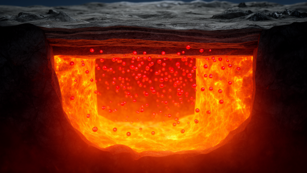
You must be logged in to post a comment.