From Watts Up With That?

By Kevin Kilty

I’d say there is no one who writes comments in threads at WUWT who doesn’t believe that radiation provides the beginning and end points of Earth’s climate. Insolation provides energy input to drive the climate, and radiation takes away waste heat at the top of atmosphere (TOA), whatever TOA means for outgoing LWIR (more about this in a moment). Figure 1 shows, using Kelvin’s statement of the Second Law of Thermodynamics, how any heat engine, climate included, must work. It must procure energy from a hot place, whether or not we can call this a reservoir in the sense of thermodynamics, or not. Some of that energy is converted to work. The remainder is discarded into a cold place, with the same statement about whether or not that is a “reservoir”.

However, there is endless discussion at WUWT, bordering on argument at times, about what goes on with regard to radiation, particularly the CO2 contribution, in the intermediate air.

The community here at WUWT are largely climate skeptics which means they tend to discount the importance of CO2. Fine. However, whether one seeks to discount or magnify the influence of CO2, one is obliged to use physically relevant arguments to do so. I hope to deep six a number of talking points that occur over and over with as rational an explanation of things as I can muster.

Transmittance measured and calculated

Let me begin with a diagram showing data collected in a laboratory. This is from the NIST website. Figure 2 shows the transmittance of IR radiation through a sample column of CO2 and Nitrogen, measured with an IR spectrometer. Transmittance is defined in terms of power transmitted by a beam of radiation. Thus, the deep troughs indicate energy per unit time that has been redirected from the beam. Where has it gone?

First, let’s examine how well a calculating engine, MODTRAN, reproduces this same picture. The pertinent parameters of the path through the sample tube in the spectrometer were 2.6 cm-atm of CO2 (the 200mmHg sample of CO2 was augmented with N2 gas to a total pressure of 600mmHg so that even the pressure broadening is representative). Figure 3 shows how the MODTRAN version at Spectral Sciences, Inc. does with parameters adjusted for 2.6cm-atm CO2.

Looks pretty close, does it not? What it says, implicitly, is that while the path length for each plotted wavelength of EM radiation contains the same concentration of CO2, we get hugely different results. Concentration doesn’t matter because the cross-section for absorption varies hugely by wavelength. Claims that CO2 can’t matter much because it is a minor chemical constituent are simply wrong.

In fact, with this version of MODTRAN I can easily check whether or not Beer’s law works. Beer’s law is defined in terms of Absorbance. Absorbance is equal to -Log(Transmittance). At a wavelength of 4.71 um, these three models of atmosphere provide the indicated transmittances:

1700cm-atm H2O, 0ppm CO2, 20km path, T=0.741

0cm-atm H2O, 400ppm CO2, 20km path, T=0.919

1700cm-atm H2O, 400ppm CO2, 20km path, T=0.708

Beer’s Law calculated for this situation is in order 0.741×0.919=0.68

And the resulting transmittance is 0.68. Comparing 0.68 to 0.708 is well within the uncertainty of all things considered. So, MODTRAN looks like a pretty solid calculator when it comes to transmittance. We will examine radiance calculations shortly, but let’s return to the NIST data. Now back to answer the question about where does this energy go?

Where does the redirected energy go?

There are really only two possible responses to the step beyond absorption. The radiant energy is either scattered into other directions other than forward, or it is absorbed by CO2 and stored as molecules with elevated energy. Scattering is nearly zero because of the size discrepancy between the EM radiation and the molecular scale. CO2 strongly absorbs radiation at the wavelengths of those deep transmittance throughs in Figure 2. Now what is the next step in the chain of conversions?

People at WUWT now claim, rightly so, that this absorbed radiation very quickly passes into the kinetic energy of nitrogen in the case of Figure 2, but into Oxygen and Nitrogen in the case of the atmosphere. This is a good thing.

Energy quickly leaves the CO2 molecules into a sea of energy shared among molecular rotations, vibrations, and speed. It is not a one-way evolution of exchanges, because down at the molecular level, what proceeds in one direction goes just as surely in the opposite, maybe at a different rate. So, evolution proceeds toward a distribution of energy by all conversion means until it is a stationary distribution – an equilibrium state. This is the Boltzmann distribution, and the atmosphere arrives there through a detailed balance of energy exchanges. Once we arrive at the Boltzmann distribution it becomes possible to speak of a “temperature” of the ensemble of molecules in near equilibrium with the sea of EM radiation within it.

I never see any reference to Boltzmann distribution, or Maxwell distribution (molecular speeds) or concept of detailed balance, even though these concepts are central to understanding both the concept of temperature (especially LTE) and radiance in the atmosphere.

The background blackbody radiation from the Earth’s surface, along with emitted radiance from nearby atmosphere, simply replaces energy lost from the local atmosphere by various means.  This sum total of interactions, and the rates at which they occur, keeps the atmosphere in local thermodynamic equilibrium (LTE).

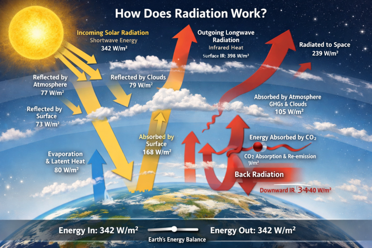
So, rather than the rapid conversion of absorbed radiation from CO2 to other molecules and other forms of energy preventing back radiation, this conversion makes possible the calculation of radiance of the atmosphere by knowing only its temperature and composition. Some of that radiance goes back to the surface.

Accurate transmission calculations, and radiance calculations from specified chemistry and temperature allow MODTRAN to act as a useful transport modeler.

A couple of other things to discuss

There is often an insistence that molecules in a cold atmosphere can’t radiate to a warmer surface because doing so would violate the Second Law of Thermodynamics. Thus, the greenhouse effect is impossible. Moreover a few people deny that a warmer instrument can measure LWIR originating from a colder place.

This insistence shows a misunderstanding of the concept of “temperature”. Molecules don’t have a temperature; they have only energy. The second law applies to temperature which is only meaningful for a large ensemble of molecules. Energy can travel anywhere, bulk heat can, spontaneously, only travel toward cold from hot, unless one forces its travel the other direction with input of work (refrigerators and heat pumps).

Another insistence by folks who overvalue CO2 is that LWIR cannot travel from the surface directly to space because it gets absorbed and much is returned to Earth. Here is how one set of professional climate scientists phrased it.

“… infrared emission from the surface is mostly absorbed in the atmosphere and cannot radiate directly to space. In turn, the atmosphere radiates both up (to space) and down (to the surface). The surface therefore receives a double whammy of radiation from both the Sun and the atmosphere…”

This represents a belief that cooling of the Earth takes place at a mythical level way up high where the temperature is 255K.

This actual level from which radiation heads to space, the cold “reservoir” that allows the atmospheric heat engine, is exceedingly complex and includes even the Earth’s surface in places and at times. Let’s use MODTRAN once again to show its two end-member clear sky models. Figure 4 shows these.

Transmittance from surface to space averaging between 14% and 32% is not negligible. Yet, there are other instances, not covered by models in MODTRAN, where average transmittance is likely higher. Portions of surface above 2,000 meters elevation, for example, are above the bulk of moist air.

The subtropics, where the furthest reach of the Hadley cell returns to Earth, is composed of air that has been substantially dried by tropical precipitation. It is very transparent to LWIR. It is also an interesting case of where dynamics and radiation meet to cooperate in cooling the Earth.   The descending air is kept warm through work performed on it by the surrounding atmospheric pressure, (or by gravity if one insists on that explanation that requires further elaboration), and radiates this work away as heat freely to space.

Even in wavelength ranges where the atmosphere is very opaque (many optical depths from surface to space) to the ballistic passage of IR radiation, there is still a flow of radiant energy that more nearly resembles diffusion, or conductive heat flow, with conductivity proportional to temperature cubed – the Rosseland approximation.

Is CO2 a negligible influence?

This essay began as a project to summarize estimates of climate sensitivity and the ways of arriving at it. However, the number of ways of arriving at that number is amazingly large. The methods have become more sophisticated over time; and more expensive! And definitions expanded the effort further by focusing on either the transient or equilibrium values. And then worrying about minor constituents of the atmosphere expanded it further, and on and on.

Soon I felt like someone auditing a Chicago election –  the accounting mattered less than who decided what details went into the accounting. However, the topic of climate sensitivity ties in well, and generates two more comments of note.

A Baseline Value of Climate Sensitivity

The effect of adding a step increase in CO2 from 400 to 800 ppm does the following. It produces a step decrease in outgoing LWIR at the top of the (tropical) atmosphere (TOA) by 3.3W/m2.[1] Obviously, the First Law of Thermodynamics applied to this situation reveals that as output is restricted a little, but insolation remains constant, the amount of stored energy in the surface and atmosphere must rise a small amount too.

Just figuring Stefan-Boltzmann (SB) feedback alone suggests a need to raise surface temperature by 0.55C to restore output at TOA. MODTRAN calculations, though, reveal that balance isn’t restored entirely by this adjustment. Through trials I find that the surface temperature must adjust by 0.76C to restore TOA balance. By this point, though, SB applied to the ground surface shows that it radiates 4.5W/m2 – 1.2W/m2 more than the simple application of SB suggests.

People have commented that this presents a paradox, “Where does the additional radiant energy come from?” The answer is that it comes back to the surface from the atmosphere. There is no paradox. It is simply the reality of dealing with boundary problems when an LWIR active atmosphere occupies the space near a boundary.

It is no different than engineers applying a coating to a surface to make an object behave thermally in a different way. This surface coating for the Earth is its atmosphere.

Now further exploration using MODTRAN is warranted because it is perfectly reasonable to suppose that increasing surface temperature will lead to increased absolute humidity with its attendant enhanced LWIR absorption.

The U of Chicago version of MODTRAN allows one to calculate the effect of a constant relative humidity with increased profile temperature. Modeling as before one finds that the surface temperature has to be increased by 1.21C to restore the original LWIR output at TOA. At this point the surface emitted energy according to SB (with emissivity=0.97) is 7.2 W/m2.

This range of values 0.76 to 1.21 centigrade, I feel, provides a useful baseline of what will happen with 2XCO2, as long as the entire process is radiation bound.

The additional comment I would make takes me back to my original motivation of look at climate sensitivity. It is a rejoinder to the often repeated reference to “Simpson and Brunt from 1938”; that atmospheric dynamics makes prediction of what 2XCO2 will do meaningless.

After Moller in 1963 spooked everyone by concluding that an atmosphere with a variable relative humidity could lead to a surface temperature that was “arbitrary[2], Manabe and Wetherald undertook an effort to model the atmosphere that was sophisticated by 1967 standards.[3] They built a model using a 1-D finite differencing algorithm that included either 9 or 18 atmospheric layers and considered the effects of clouds, CO2, ozone, and water vapor either in constant RH or constant vapor pressure models. Their effort was complicated at this time because in addition to addressing the long-time worry over CO2 warming, there was an additional worry over the SuperSonic Transport (SST) adding water vapor to the stratosphere. What they found, however, was that reasonable distributions of absolute humidity would lead to 1.3 degrees centigrade warming while reasonable assumptions about relative humidity would lead to 2.3 degrees centigrade.

Spencer and Christy [4] (also open access) describe the construction of a 1-D model of vertical heat transport starting with the deep ocean and proceeding through the atmosphere. Their model involves three oceanic layers, three atmospheric layers. Having made this model and verifying it. They then considered estimates of energy imbalance made in various ways (satellite radiometery, Argo floats, borehole measurements, etc) and determined what climate sensitivity values produce a consistent story between energy imbalance, their 1-D model, and observed Earth temperatures since either 1970 or 1850 depending on data source, and also consistent with the two-sigma uncertainties in all quantities.

Their results range from 1.86 to 2.49 degrees centigrade per doubling of CO2. Lewis and Curry (2018)[5] found similar values using similar means. Three dimensional computer climate models produce greater climate sensitivity estimates (up to 5K) still. Yet then using these exact codes within the context of Earth system models produce much less warming (3.3K).[6] It is as though one can’t get a reasonable value of climate sensitivity without including every influence from the biosphere, cryosphere, oceans and atmosphere, because then one misses significant negative feedbacks. But in answer to Simpson and Brunt, despite many attempts to determine climate sensitivity in various ways, nothing seems lower than my baseline from radiation alone.

Notes:

1-The range of values for the decline in outgoing LWIR is 1.8 to 3.5 W/m2 through the full suite of MODTRAN models. Not as great as the Tropical model value, but not insignificant either.

2- F. Möller, On the influence of changes in the CO2 concentration in air on the radiation balance of the Earth’s surface and on the climate, Journal of Geophysical Research, 1 July 1963 https://doi.org/10.1029/JZ068i013p03877

3-Syukuro Manabe and Richard T. Wetherald, Thermal Equilibrium of the Atmosphere with a Given Distribution of Relative Humidity, Journal of the Atmospheric Sciences,  Page(s): 241–259, 01 May 1967 DOI: https://doi.org/10.1175/1520-0469

4-Roy W. Spencer and John R. Christy, Effective climate sensitivity distributions from a 1D model of global ocean and land temperature trends, 1970–2021, Theoretical and Applied Climatology (2024) 155:299–308

Effective climate sensitivity distributions from a 1D model of global ocean and land temperature trends, 1970–2021 | Theoretical and Applied Climatology | Springer Nature Link

5-Nicholas Lewis and Judith Curry, 2018, The Impact of Recent Forcing and Ocean Heat Uptake Data on Estimates of Climate Sensitivity, Journal of Climate,  6051–6071

DOI: https://doi.org/10.1175/JCLI-D-17-0667.1

6-See for instance at The Geophysical Fluid Dynamic Lab and note the table of models.

For those wishing to pursue some challenging explanation of LTE:

Hermann Harde, Radiation and Heat Transfer in the Atmosphere: A Comprehensive Approach on a Molecular Basis, International Journal of Atmospheric Sciences, 27 October 2013 https://doi.org/10.1155/2013/503727